
A few strong to marginally severe thunderstorms are possible across the Southeast U.S. Friday. A Marginal Risk (Level 1 of 5) outlook has been issued. Strong winds and hail will be the main threats. Elevated to locally critical fire weather conditions will persist across south-central Colorado today due to dry conditions and gusty winds. Read More >
The 21 February 1997 High Shear/Low CAPE Severe Weather Outbreak
Justin D. Lane

1. Overview
A persistent, shallow (i.e., storm tops less than 20.0 kft) quasi-linear convective system (QLCS) produced widespread straight line wind damage and several tornadoes (Appendix A) across northeast Georgia, Upstate South Carolina, and the Piedmont of North Carolina between 1900 UTC and 2300 UTC on 21 February 1997. The tornadic storms on this day were generally accompanied by the “broken-S” radar reflectivity signature.
2. Large Scale Environment
Hydrometeorological Prediction Center (HPC) reanalysis data at 1800 UTC on 21 February 1997 showed a deep trough over the central United States (Fig. 1). At the surface, low pressure was located over Indiana and Illinois, with a cold front inferred from the western Ohio Valley through the lower and middle Mississippi Valley. A strong and deep jet stream was evident across much of the Ohio and Tennessee Valleys.
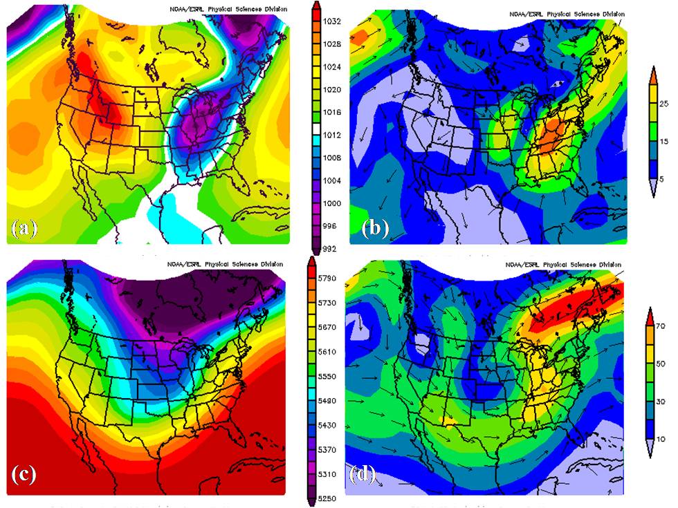
Fig. 1. HPC reanalysis of (a) Sea level pressure (hPa) (b) 850 hPa wind (m s-1) (c) 500 hPa geopotential height (m) and (d) 300 hPa wind (m s-1) at 1800 UTC on 21 February 1997.
The 1200 UTC observed sounding from Birmingham, Alabama (Fig. 2) was chosen as the sounding most likely representative of the atmospheric conditions over the area of concern at the time of the outbreak. Convective Available Potential Energy (CAPE) calculated using the most unstable parcel in the sounding (MUCAPE) was 181 J kg-1. Roughly one-third of the CAPE (38 J kg-1) was contained within the lowest 3 km. Winds in the lower troposphere were very strong, with a deep layer of 55 kt to 65 kt wind observed in the 1 km to 6 km layer. This resulted in strong wind shear, especially in the lower levels, where it was calculated at 27 m s-1 in the 0-3 km layer. The clockwise curvature in the hodograph was evidence of impressive storm relative helicity of 540 m2 s-2 in the lowest 3 km.
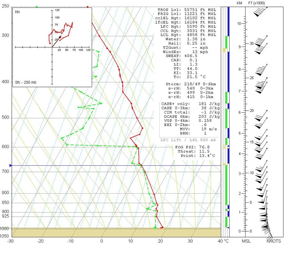
Fig. 2. Skew-T/log p diagram for the observed upper air sounding from Birmingham, AL at 1200 UTC on 21 February 1997. The air temperature trace is shown by the solid red line and the dewpoint temperature trace is shown by the dashed green line.
3. Convective Evolution
A shallow, narrow line of convection moved across north Georgia during the afternoon, resulting in fairly widespread wind damage. A four-panel display from the Greer, SC (KGSP) WSR-88D at 1933 UTC on 21 February 1997 (Fig. 3), near the time of onset of an area of damage across northwest Hall County, showed a break in a QLCS between Dahlonega and Gainresville. Although this damage was described as straight-line wind in Storm Data (with some damage attributed to “gustnadoes”), the reflectivity data fits very well with the conceptual model of broken-S tornadoes (Fig. 4.). Previous studies of broken-S events (i.e., McAvoy et al., 2000, Lane and Moore 2006) indicated that the tornado occurred in association with an appendage on the lower (i.e., southern) tip of the reflectivity segment on the cyclonic shear side (i.e., to the north) of the causative rear inflow jet.
Another apparent tornado developed in extreme northeast Hall County and continued into southern Habersham County, Georgia after 1945 UTC. The damage was described in Storm Data as straight line winds, with embedded gustnadoes in Hall County, but as tornadic in Habersham County. While the northwest Hall County event was associated with a very distinct broken-S signature, the signature associated with the later event was much more subtle (Fig. 5).
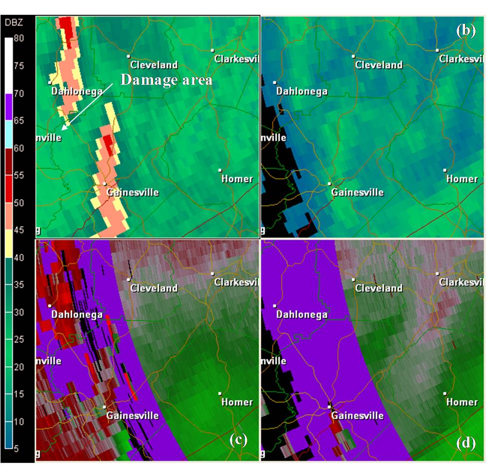
Fig. 3. Images of (a) base reflectivity at 0.5 degrees, (b) base reflectivity at 1.5 degrees, (c) storm relative velocity at 0.5 degrees, and (d) storm relative velocity at 1.5 degrees from KGSP.
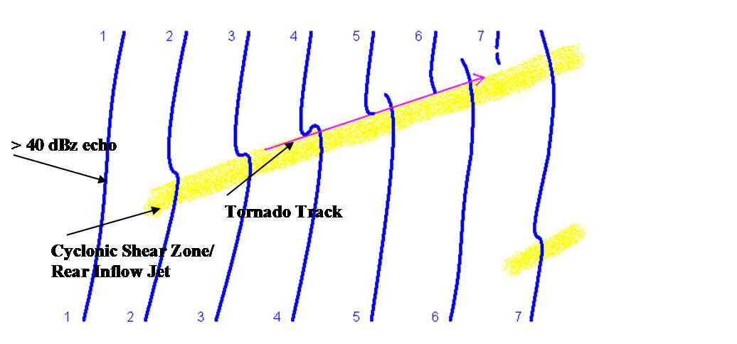
Fig. 4. Conceptual model of time series of broken-S evolution. Each time step represents a new radar volume scan. Note: the tornado may occur at any time after frame 3.
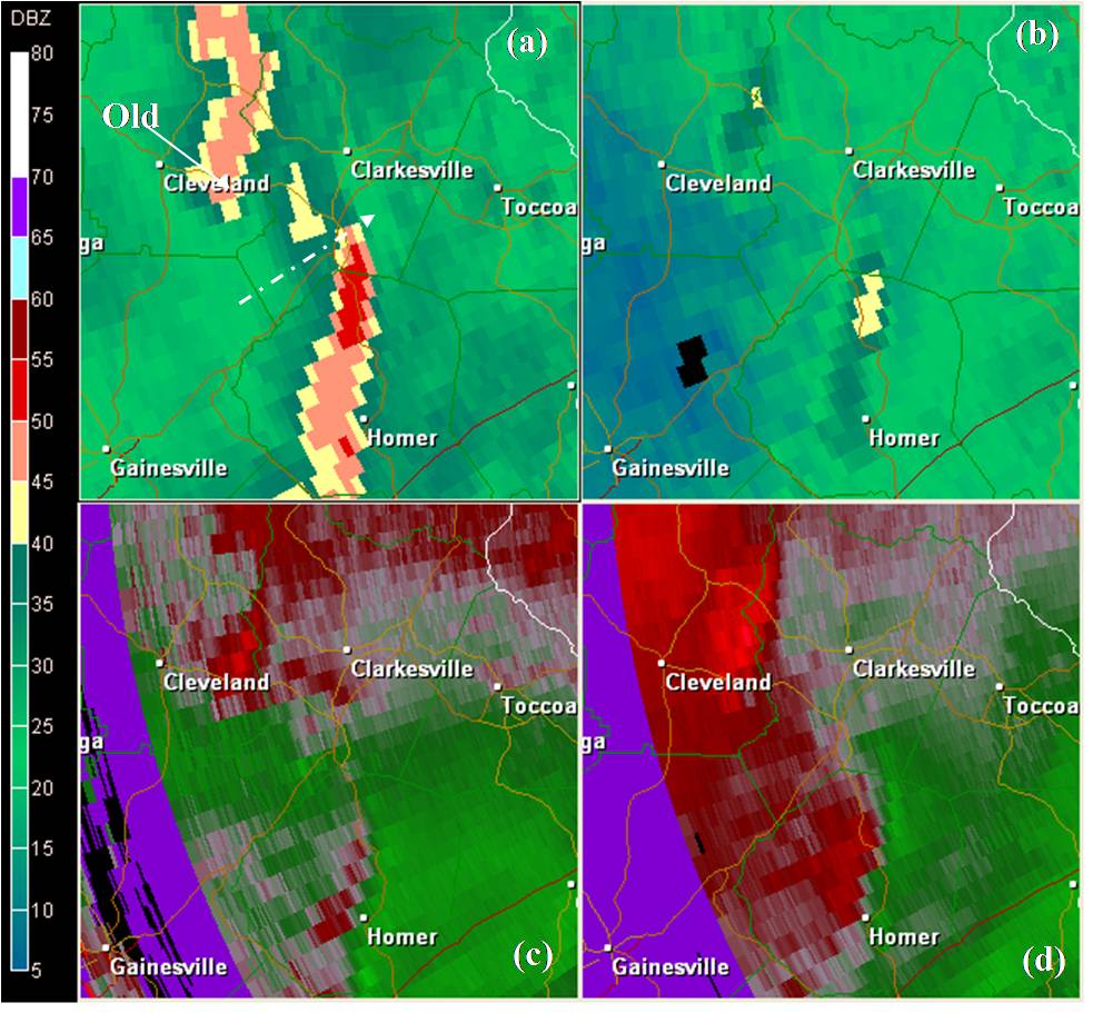
Fig. 5. Same as in Fig. 3 except at 1951 UTC. The approximate tornado path is denoted by the dashed arrow. The segment responsible for the earlier Hall County tornado is labeled “Old.”
As the QLCS moved rapidly to the east-northeast, a very brief, weak tornado (F0) occurred in Oconee County, South Carolina at around 2020 UTC. The radar signature associated with this event was even more subtle than with the previous tornado. In fact, the reflectivity signature could hardly be deemed a “broken-S,” although there was a channel of weak reflectivity (i.e., less than 40 dBz) noted across the line segment at 1.5 degrees (Fig. 6). It is also interesting to note that the linear segment associated with the earlier northwest Hall County tornado was producing significant straight line wind damage over Oconee County south of Walhalla at around this time.
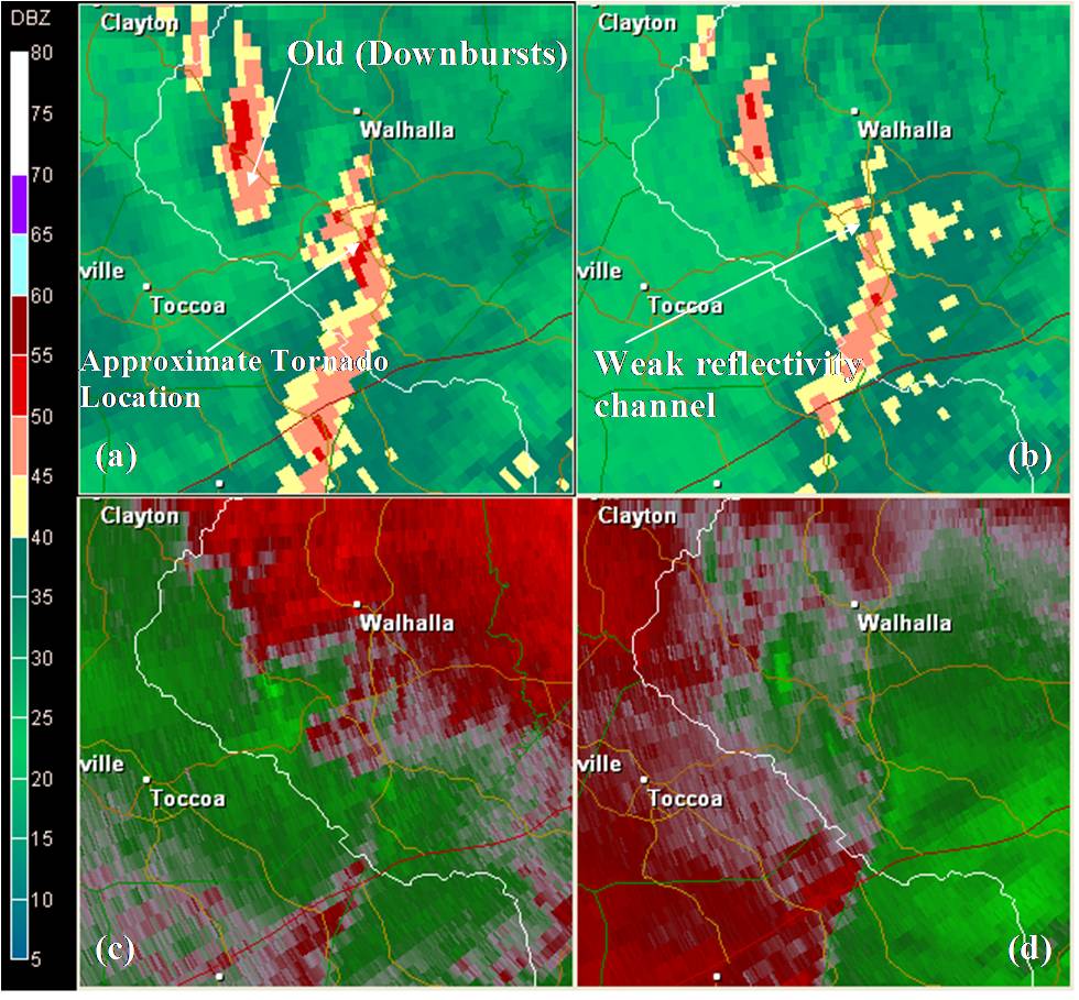
Figure 6. Same as in Fig. 3 except at 2020 UTC.
As the QLCS progressed (SRM loop) across Upstate South Carolina, severe weather occurrence shifted further south along the line. Another weak tornado occurred just west of the Honea Path community just after 2100 UTC. Although this event was associated with a pronounced bow echo reflectivity structure, a broken-S pattern was not identified (Fig. 7). However, there was a pronounced rear inflow notch observed in the 2.4 degree (7.7 kft AGL) and 3.4 degree (10.2 kft AGL) elevation slices just before tornado occurrence. This notch descended with time (Fig. 9).
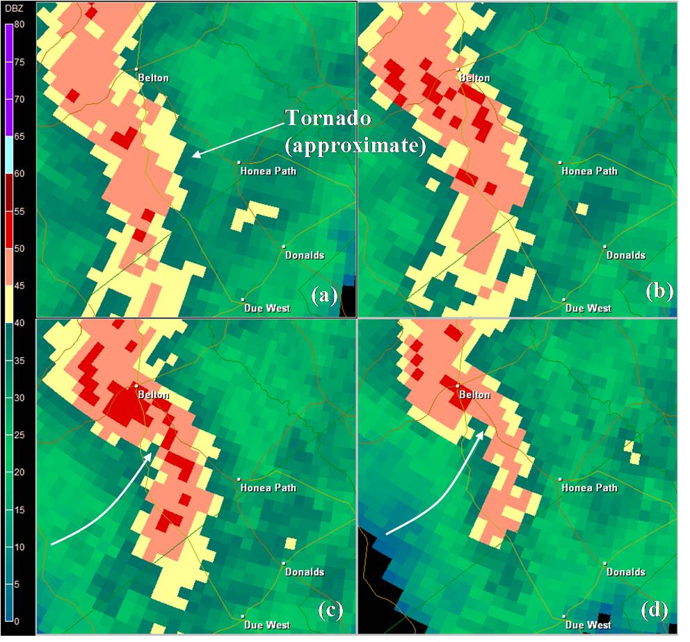
Figure 7. Reflectivity images at (a) 0.5 degrees, (b) 1.5 degrees, (c) 2.4 degrees, and (d) 3.4 degrees at 2100 UTC on 21 February 1997. The arrows are oriented along the rear-inflow notch.
The storm relative velocity at 2100 UTC (Fig. 8) revealed classic bow echo structure. The presence of a rear inflow jet was confirmed with an area of relative enhanced inbound velocity behind the gust front. Meanwhile, there was an area of cyclonic shear through the lowest 10.0 kft AGL that narrowed and weakened toward the ground. However, this vortex was located several miles north of the reported[1] tornado location, north of and adjacent to the rear inflow jet. What, if any role this vortex played in tornadogenesis is unknown.
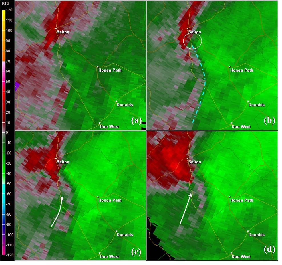
Fig. 8. Same as in Fig. 7 except for storm relative velocity. The gust front is denoted by the dashed blue line. The white circle outlines the book-end vortex.
As the bow echo associated with the Honea Path tornado decayed, the most active portion of the QLCS (SRM loop) shifted back to the northern end of the line. The most intense tornado (F2) on this day occurred at around 2130 UTC near the city of Spartanburg. Once again, the reflectivity data from this time did not reveal a well-developed broken-S structure, at least in the lowest 7000 feet or so (Fig. 10). However, a broken-S pattern was noted in the higher elevation scans (6.2 degrees; 10.1 kft). The broken-S pattern did extend to the lower elevation slices in subsequent radar scans (Fig. 12). However, this was after the tornado had dissipated. This event and the Honea Path event provided anecdotal evidence that tornadogenesis was closely tied to the descent of a rear-inflow jet.
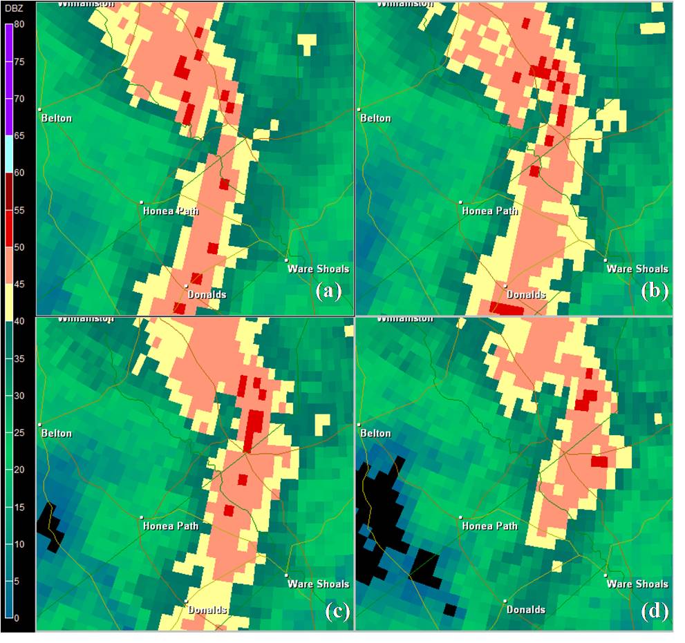
Fig. 9. Same as in Fig. 7 except at 2111 UTC.
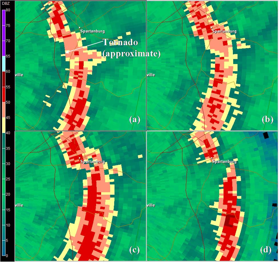
Fig. 10. KGSP base reflectivity at (a) 0.5 degrees, (b) 2.4 degrees, (c) 4.3 degrees, and (d) 6.2 degrees at 2130 UTC on 21 February 1997.
The storm relative velocity image from around the time of the tornado (Fig. 11) revealed an area of cyclonic shear near the area where the tornado occurred. However, the shear was broad and quite weak (rotational velocity of around 25 kt). It was somewhat surprising that a stronger rotational couplet was not observed, since the tornado occurred only 14 nm from the KGSP radar. However, the tornado apparently occurred a minute or two before these images, and was very brief (less than a minute duration). A tornado vortex signature (TVS) may have been observed if the radar had sampled the cell during the time of the tornado.
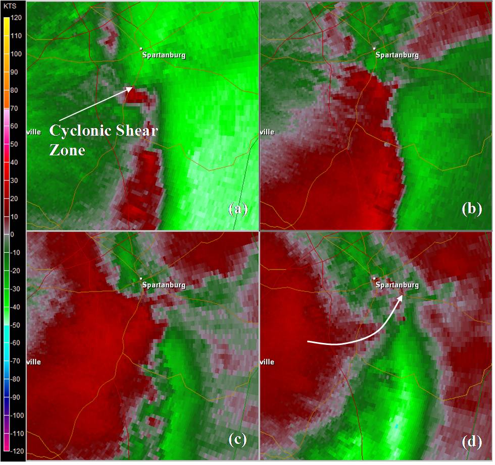
Fig. 11. Same as in Fig. 10, except storm relative velocity.
After the Spartanburg tornado, there was a relative lull in tornadic activity. However, there was an apparent increase in intensity of downburst damage between 2130 and 2200 UTC. The reflectivity images from 2146 UTC revealed the remnant broken-S structure west of Gaffney that developed in association with the Spartanburg tornado. However, damage during this time was apparently confined to areas south along the line, between Gaffney and Union, where some structural damage occurred. Although there was a slight bowing structure to the QLCS, there was a general absence of notable storm-scale features during this time, despite the ongoing severe weather. However, convection was relatively deep, with high reflectivity cores (i.e., > 50 dBZ) extending as high as 15 kft, among the highest observed on this day. It is possible that these deeper reflectivity cores were mechanically mixing the very high momentum air from aloft to the surface. This downward momentum may have been augmented via microphysical processes (i.e., melting ice). The base velocity data at 2146 UTC (Fig.13) showed a broad area of very high outbound velocities (55 kt to 70 kt) at an elevation as low as 1.7 kft AGL in the vicinity of the QLCS that extended rearward from the gust front.
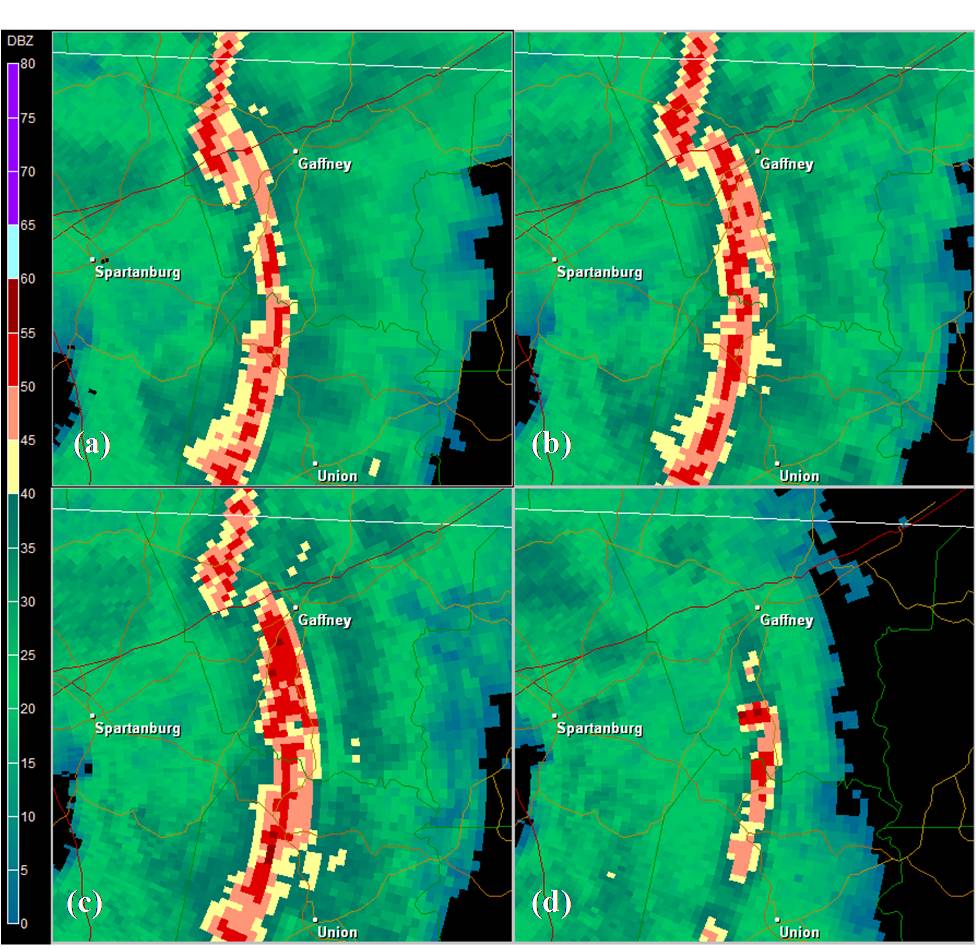
Fig. 12. KGSP base reflectivity at (a) 0.5 degrees, (b) 1.5 degrees, (c) 2.4 degrees, and (d) 4.3 degrees at 2146 UTC on 21 February 1997.
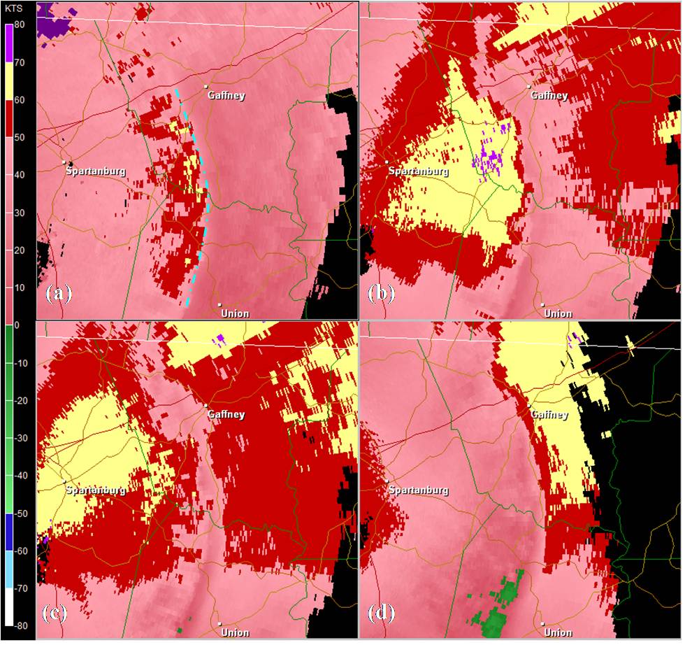
Fig. 13. Same as in Fig. 12 except base velocity. The dashed blue line delineates the approximate location of the gust front.
One final tornado, which was weak (F1) but fairly long-lived, developed in association with the QLCS as it moved into the North Carolina Piedmont. This event was similar to the first Hall County, Georgia, tornado in that it occurred in association with a well-defined broken-S signature (Figs. 14 and 3). Once again, the “broken-S” structure developed from the top-down, indicating that it was associated with a descending rear inflow jet. This was another event that conformed to the conceptual model of the broken-S signature as described earlier in this section.
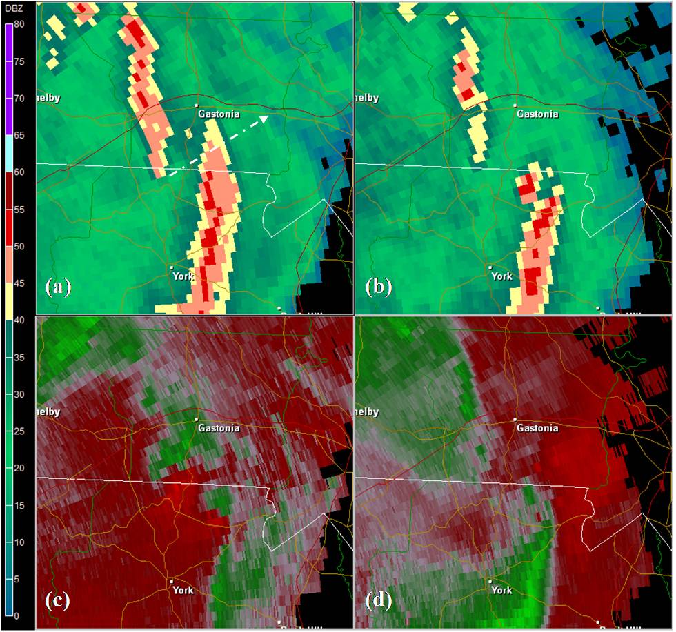
Fig. 14. Same as in Fig. 5 except at 2217 UTC. The dashed arrow represents the approximate tornado path.

Fig. 15. Same as in Fig. 5 except at 2227 UTC.
4. Summary
A long-lived, shallow QLCS produced widespread wind damage, several weak tornadoes, and one strong tornado as it moved across north Georgia and the Piedmont of the western Carolinas during the afternoon of 21 February 1997. Although the QLCS exhibited classic bow echo structure (pronounced rear inflow notches, book-end vortices) from time to time, these features were generally not long-lived. Nevertheless, widespread and persistent wind damage was observed along the length of the QCLS throughout most of its lifetime. Because wind damage, some of which was significant, occurred even in the absence of classic storm scale features, convective mixing of very high momentum air from aloft may have played a key role in damaging wind occurrence. When bow-echo features did develop within the QLCS, they were often accompanied by rapid tornadogenesis. Recent research (i.e., Atkins and St. Laurent, 2008; Weisman and Trapp, 2003) has shown that intense low-level mesovortices can develop within QLCS in strongly sheared environments as the rear inflow jet descends. Most of the tornadoes that occurred on 21 February 1997 were associated with the broken-S reflectivity signature. The broken-S pattern was typically first observed in the mid-levels of the QLCS (i.e., 7.0 kft to 12.0 kft), but then descended rapidly toward the surface in subsequent volume scans, suggestive of a descending rear-inflow jet. As has been observed in other studies, and as suggested by the schematic in Fig. 4, some of the tornadoes occurred well before the fully-formed broken-S was observed at the lowest elevation scans, while some occurred after the signature was identified. This phenomenon may be a simple matter of radar sampling. In other words, the signature may typically develop first in the mid and upper levels of the QLCS, and then descend toward the surface. Therefore, if the storm is at a relatively large distance from the radar, the “break” may only be visible at the lowest elevation scan. Meanwhile, QLCS that are within close proximity of the radar may exhibit a break first at higher elevation scans, with the signature appearing in the lowest scan near the time of tornadogenesis, or even after the tornado has occurred. It is therefore important for operational forecasters to perform a complete vertical assessment of QLCS structure during high shear/low CAPE environments.
Acknowledgements
All radar imagery was created using GRLevel2 software. The sounding was created with the Universal RAwinsonde OBservation (RAOB) Program. Reference to any specific commercial products, process, or service by trade name, trademark, manufacturer, or otherwise, does not constitute or imply its recommendation, or favoring by the United States Government or NOAA/National Weather Service. Use of information from this publication shall not be used for advertising or product endorsement purposes.
References
Atkins, N.T. and M. St. Laurent, 2009: Bow Echo Mesovortices. Part II: Their Genesis. Mon. Wea. Rev., 137, 1514-1532.
Lane, J. D., and P. D. Moore, 2006: Observations of a non-supercell tornadic thunderstorm from a Terminal Doppler Weather Radar. Preprints, 23rd Conf. on Severe Local Storms, St. Louis, MO, Amer. Meteor. Soc.
McAvoy, B. P., W. A. Jones, and P. D. Moore, 2000: Investigation of an unusual storm structure associated with weak to occasionally strong tornadoes over the Eastern United States. Preprints, 20th Conf. on Severe Local Storms, Orlando, FL, Amer. Meteor. Soc., 182-185.
Weisman, M. L., and R. J. Trapp, 2003: Low-level mesovortices with squall lines and bow echoes. Part I: Overview and dependence on environmental shear. Mon. Wea. Rev., 131, 2779-2803.
[1] It should be noted that details on the exact location (i.e., roads affected, etc.) of the tornado are absent in Storm Data. The location listed in Storm Data (2 W Honea Path) cannot be independently verified.


 Current Conditions Map
 Follow us on YouTube