-
What is HL-RMS?
Modeling framework for testing lumped, semi-distributed, and fully-distributed
hydrologic modeling approaches.
-
HL-RMS Components
-- Current computational element: NEXRAD 4km grid;
-- Rainfall/runoff modleing in each element;
-- Computes hydrographs at any interior point;
-- Uses lumped or distributed model parameters;
-- Uses lumped or distributed precipitation;
-- Ingests NEXRAD Stage III xmrg data;
-- Hillslope, channel routing: kinematic;
-- Modular design to test other models;
-- Uses connectivity matrix.
-
Brief Description of HL-RMS
As a DMIP initiative, HL has developed the first version of a Research
Modeling System (HLRMS) that combines lumped and distributed model features.
While the system has a grid-based structure, it can be run in lumped or
semi-distributed modes. The main goal of the HLRMS was to generate a flexible
system that can easily incorporate different parameterizations of rainfall-runoff
and routing processes. All parameterizations should be identifiable based
on GIS and hydrological data.
System structure and hydrologic models are described as
follows:
The first version of the HLRMS is consistent with an HRAP projection,
such as computational elements are defined on a sequence of HRAP pixels.
Each element consists of a rainfall-runoff component (in version 1 - SAC-SMA
model) and a routing component (in version 1 - hillslope/channel kinematic
wave model). Rainfall-runoff component generates fast (surface) and slow
(subsurface/ground) runoffs. Within each element, a fast runoff is routed
over conceptual hillslope to a channel, and then channel inflow combined
with a slow runoff component and upstream pixel outflows is routed through
a pixel conceptual channel. A conceptual hillslope consists of a number
of uniform hillslopes (a number of hillslopes depends on a stream channel
density of a pixel). A conceptual channel usually represents the highest
order stream of selected pixel. Cell-to-cell connectivity
sequence must be determined to move water from upstream to downstream
elements and to a basin outlet. An implicit numerical scheme is used for
kinematic equation solution.
Data format for input variables and model parameters are similar to
'xmrg' binary type grids with a minor difference in the header. All parameter
grids are binary files with two header records. The first record is the
same as the 'xmrg' record that consists of X- and Y-orifins of HRAP, and
numbers of columns and rows in the file. The second record differs from
‘xmrg' records. It includes two variables: scale factor to convert integer*2
values into real values, and number of bytes per value (2 for integer*2
format, and 4 for real*4 format). This allows to keep grids in integer*2
or real*4 formats. In the first run, the model will read archived ‘xmrg'
files directly. In the same time, a separate new binary file will be created
for each selected non-nested basin. These new binary files contain precipitation
data only for those grids contained in the selected basins. It will greatly
reduce the run-time for further model test runs. State variables will be
saved as the same format as newly created precipitation data except that
they are corresponding to a specific time. During the run time, all grids
are converted into one-dimensional arrays in a pixel connectivity order.
A number of separate or nested basins can be processed simultaneously.
Hydrographs at selected outlets are stored in an OH card format. Selected
grids (input variables, states, water balance components) can be stored
in an Arc/Info format for a selected period with desirable time interval.
Input variables. Precipitation 'xmrg' hourly grids. Climatological
monthly evapotranspiration demand and PE adjustment factor grids. NOTE:
Hourly/daily potential evaporation grids can be also used if available.
Initial state variables. Six SAC-SMA upper-lower zone
states (UZTWC, UZFWC, LZTWC, LZFSC, LZFPC, ADIMPC), hillslope routing state
(water depth of each pixel), and channel routing state (channel cross-section
at each pixel) grids.
Parameters. 16 SAC-SMA parameter grids. Hillslope slope,
roughness coefficient, and stream channel density grids. Channel slope,
roughness coefficient, shape parameter, b, and top width parameter, a,
grids. Shape and top width parameters are defined based on a relationship
between channel top width and depth, B=a*H**b. The program
converts hillslope parameter grids into one basic hillslope parameter grid,
a specific hillslope discharge per a unit depth. Four channel grids are
converted into two basic channel parameter grids, a specific channel discharge
per a unit channel cross-section, and a power value in relationship between
discharge and cross-section.
Grid replacement and adjustment. All variable and parameter
grids except precipitation can be replaced by some uniform values for each
selected basin/subbasin. They can be also adjusted by some ratio for each
selected basin/subbasin. An information on replacement or adjustment is
provided in an input deck of the HLRMS .
-
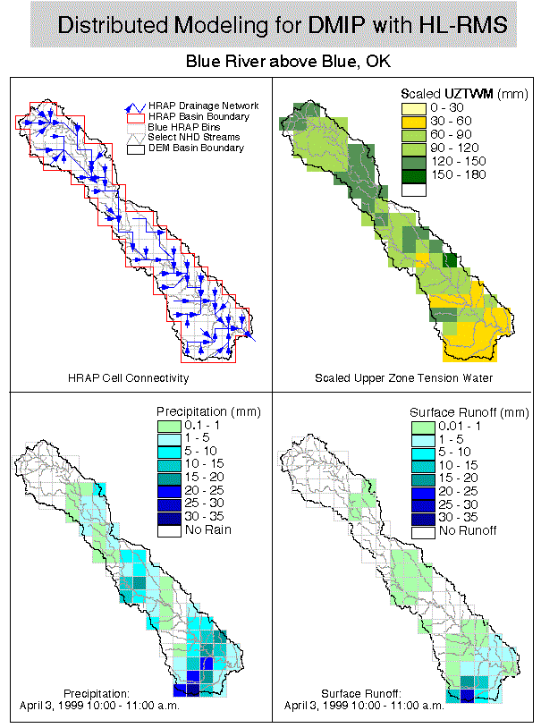
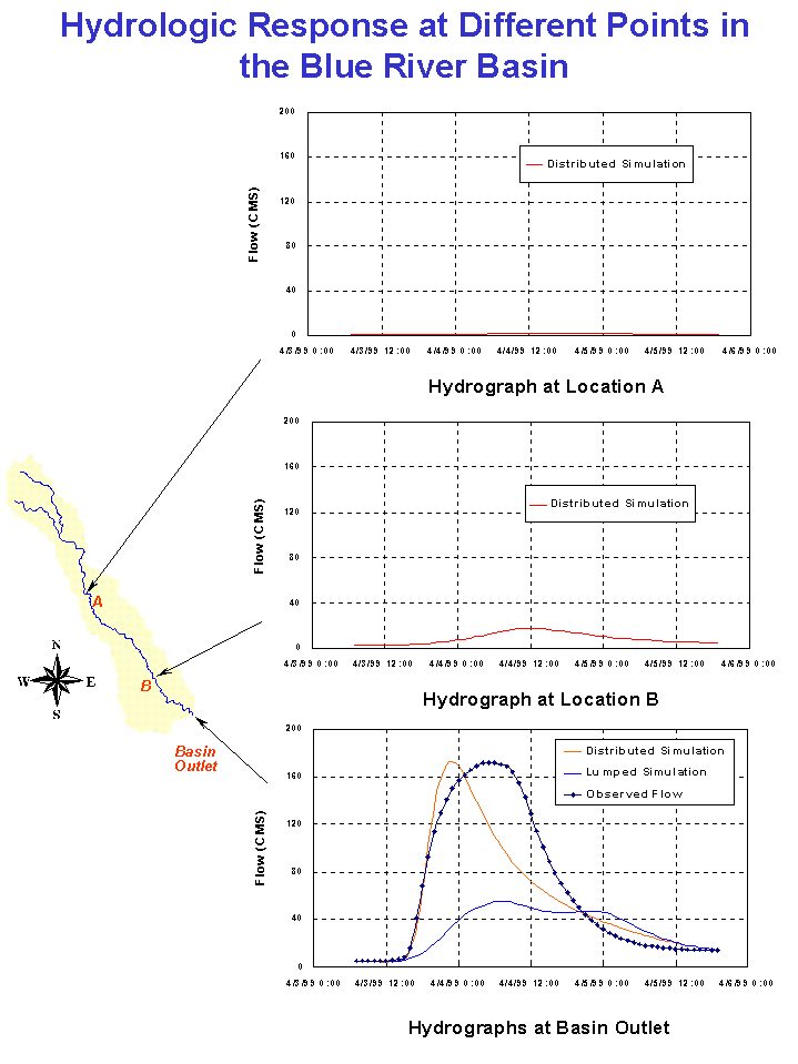
Example Simulation From HL-RMS