|
The Alabama gravity wave event of February 22, 1998: A classic mesoscale forecasting challenge John T. Bradshaw, Ronald A. Murphy, and Kevin J. Pence 1. INTRODUCTION On the morning of 22 February 1998, much of Alabama was unexpectedly rocked by a period of intense sustained wind, estimated at times in excess of 31 ms-1 (60 knots). Moving rapidly northward across the state in a wide band, the strong winds produced squall-like conditions which lasted roughly 10 to 20 minutes at individual locations. Shingles were ripped off of dozens of roofs, and large trees were toppled onto houses, cars, and roads throughout the Birmingham metropolitan area. Structural damage and power outages were widespread across the remainder of central and northern Alabama. Examination of Automated Surface Observing System (ASOS) 1-minute frequency pressure and wind observations, as well as regional rawinsonde sounding data suggest that the strong winds were the result of a large-amplitude mesoscale gravity wave, which likely originated in the northwest Gulf of Mexico and moved northward across Alabama. Extraordinarily large pressure fall rates of up to 35 hPa hr-1 accompanied the strong winds at several ASOS sites. Regional WSR-88D reflectivity products depicted a wide band of moderate to heavy precipitation which traveled northward across Alabama during the morning hours of 22 February. A comparison of ASOS and radar data reveals that the mesoscale wave was located anywhere from 5 to 40 km behind the trailing edge of the precipitation area, and was moving in tandem with it. At each location, the onset of the strongest winds coincided with the cessation of the precipitation, and occurred during the period of greatest pressure falls. The large-scale meteorological pattern present during this event was consistent with those of other significant gravity wave cases (e.g., Koch and Dorian 1988; Schneider 1990; Ramamurthy et al. 1993), and fits the conceptual model for mesoscale gravity wave formation proposed by Uccellini and Koch (1987). In particular, the wave activity occurred to the northeast of a deepening surface low, and north of a warm frontal boundary. Additionally, the highly diffluent right exit region of a 300 hPa jet maximum was juxtaposed on the wave track. The gravity wave likely originated as part of a geostrophic adjustment process occurring in response to force imbalances within the upper-level jet streak. Area soundings and model data revealed the presence of a suitable low-level duct which allowed the excited wave to propagate northward across Alabama for several hours. 2. LARGE SCALE CONDITIONS
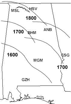
Figure 1 depicts the surface pressure and temperature patterns at 1200 UTC on the morning of 22 February 1998. A strong low pressure area was centered over southern Louisiana, with a warm front extending eastward over the northern Gulf of Mexico. An easterly flow prevailed over most of Alabama, with most stations reporting wind speeds ranging from 5 to 10 ms-1 (10 to 20 knots) during the period of the gravity wave event. Aloft, a strong diffluent trough was moving eastward out of Texas into the lower Mississippi Valley, accompanied by a vigorous mid-level vorticity maximum over the western Gulf of Mexico. Downstream from the trough, an amplified ridge covered most of the eastern United States. At 300 hPa (Fig. 2), a 40 ms-1 jet streak was propagating northeastward through the front side of the trough toward the inflection point of the downstream ridge. Not surprisingly, the dynamic system was producing strong quasi-geostrophic (QG) upward motion across portions of the Deep South during this time period. Significant deep layer Q-vector convergence (implying ascent) was present along the upper Gulf Coast (not shown), and was migrating northward. In response to this broad region of lift, precipitation developed over most of southern Alabama prior to 1500 UTC, and advanced rapidly northward in concert with the synoptic scale forcing. 3. WAVE OBSERVATIONS 3.1 ASOS wind speed and pressure observations Compelling evidence for a mesoscale wave disturbance is seen in the ASOS data on the morning of 22 February. Figure 3 depicts the locations of 6 ASOS sites in Alabama and west central Georgia for which 1-minute data are available. Plots of wind speed and station pressure observations from 3 of these sites are shown in Fig. 4. Each of these plots represents a one hour window encompassing the wind event at each site. The wave first appears at Evergreen (GZH) at 1503 UTC (Fig. 4a). The station pressure begins to fall steeply at this time, ultimately dropping 7.8 hPa during the next 30 minutes. Coincident with this pressure fall, wind speeds increase sharply from an average of 6 ms-1 (12 knots) at around 1500 UTC to 17 ms-1 (34 knots) by 1522 UTC. The wind maintains this intensity for approximately 8 minutes, then diminishes to near 10 ms-1 (20 knots) by 1550 UTC. A pressure minimum occurs at 1533 UTC, followed by a small recovery during the next 30 minutes. A similar sequence of events occurs about an hour later at Montgomery (MGM), located approximately 108 km northeast of GZH. A steep pressure fall occurs between 1600 and 1635 UTC (Fig. 4b), resulting in a total pressure change of 8.4 hPa. Wind gusts at MGM are stronger than at GZH, peaking around 20.6 ms-1 (40 knots) at 1629 UTC. Shortly after this time, the first structural damage occurs in two separate counties northwest of Montgomery. The wave next appears at Birmingham (BHM), where it produces the steepest pressure falls, highest wind speeds, and greatest concentration of damage. As depicted in Fig. 4c, an extremely steep pressure fall of 9.9 hPa occurs at this site in just 17 minutes! Wind speeds intensify rapidly in conjunction with the pressure change, rising from an average of 11 ms-1 at 1650 UTC to nearly 20 ms-1 (40 knots) by around 1709 UTC. The high wind speeds are maintained for about 10 minutes, followed by a slight lull between 1720 and 1728 UTC. A second period of stronger winds then commences, culminating in a peak gust of 22.7 ms-1 (44 knots) at 1739 UTC. The terrain in the Birmingham area is quite varied, with some of the ridges along the southern periphery of the city rising as much as 152 m (500 feet) above the elevation of the BHM ASOS. These elevated areas, which in many cases were aligned normal to the prevailing east wind direction during the event, had much greater exposure to the higher winds in the boundary layer. As a result, most of the structural damage occurred in the residential neighborhoods lining the crests of these ridges. In some cases, the nature of the damage (e.g., large trees toppled, numerous shingles removed) was consistent with wind gusts in excess of 30 ms-1 (~ 60 knots). Following wave passage at BHM, the feature is observed shortly afterwards at Columbus, GA (CSG), Anniston, AL (ANB), and Muscle Shoals, AL (MSL). A similar evolution in the pressure and wind speed data occurs at each of these locations; rapid pressure falls of 5.0 to 8.5 hPa are accompanied by sustained winds of 14 to 18 ms-1 (28 to 35 knots). The last ASOS site in Alabama to experience the wave is Huntsville (HSV), where a steep pressure drop concludes around 1810 UTC, or roughly 3 hours after the wave's first appearance at GZH.
3.2 Radar observations As noted previously, a large precipitation area developed over southern Alabama early on the morning of 22 February and migrated rapidly northward across the state. Figure 5 (refer to Satellite/radar images and loops.) depicts the progress of this precipitation as observed by area WSR-88D radars during the period from 1446 to 1814 UTC. Most of the precipitation appears to be stratiform in nature, given the non-cellular appearance and modest reflectivity values of 30 to 40 dBZ However, some weak elevated instability was apparent in area soundings at 1200 UTC, and the arrival of strong upward motion likely further increased the mid-level lapse rates across the region. As a result, a few thunderstorms did develop over central and eastern Alabama within the larger scale rain mass, as confirmed by reports of thunder at KMGM and KCSG. Reflectivities with these storms exceeded 50 dBZ at times, although their appearance was not at all suggestive of severe convection in general, or specifically a squall-line, which might otherwise account for the wind and pressure features observed in the ASOS data. 3.3 Wave location and movement Unfortunately, insufficient ASOS observations were available to perform either a time to space conversion or a cross-spectral analysis of the pressure perturbation data, as discussed by Koch and O'Handley (1997, hereafter KO97). This type of analysis would likely pinpoint the locations, amplitude, and phase velocity of the wave disturbance. However, a crude assessment of the wave's motion can be made by considering the relationship between the times of precipitation cessation and minimum pressure at each ASOS site. Precipitation ending times can be deduced by examining WSR-88D reflectivity products (Fig. 5 refer to Satellite/radar images and loops.), and noting the time at which the back edge of the rain band (defined as the 20 dBZ contour) reaches each location. Initially, the wave trails the back edge of the reflectivity by 25 and 14 minutes at GZH and MGM, respectively. However, by the time the wave reaches BHM, CSG, ANB and MSL, it lags the precipitation area by only 3 to 5 minutes. Assuming the time rate of change of distance between the precipitation and the wave is linear, one can estimate the isochrones of the pressure trough, as shown in Fig. 3. Initially, the wave appears to be roughly planar in shape as it moves out of southwest Alabama. However, over time it assumes a double-arc shape, suggesting that the wave may actually consist of two non-planar waves. Based on the positions of the wave arcs from 1600 to 1800 UTC, the phase velocity (C) of the wave group is estimated at 28 ms-1, and the direction of movement is from 220o. KO97 proposed an alternative means of estimating C,using the mean wind vector within the unstable layer. Employment of this technique with the KBMX rawinsonde sounding from 22 February 1200 UTC (Fig. 6) yields a wave motion of 217 at 28.7 ms-1, which agrees quite well with the manually-derived estimate. 4. WAVE GENESIS AND MAINTENANCE MECHANISMS Several mechanisms have been proposed to explain the formation of large amplitude mesoscale gravity waves. In particular, Uccellini and Koch (1987) and KO97 extensively discuss the role of geostrophic adjustment arising from unbalanced flow in the exit regions of upper level jet streaks. As described by KO97, a measure of this unbalanced state can be obtained by calculating a Lagrangian Rossby number (RoL), which is the ratio of the component of the ageostrophic wind directed across height contours, to the total wind. Values of RoL > 0.5 imply large amounts of cross-contour ageostrophic flow, brought about by parcel deceleration in the highly diffluent exit regions of upper jets. Ageostrophic flow toward the cyclonic side of the jet streak violates the concept of QG theory, thereby indicating an unbalanced state and a potential for gravity wave development. The ETA 300 hPa analysis at 1200 UTC (Fig. 2) depicts a robust cyclonically curved jet streak extending from southern Texas into central Louisiana, with a highly diffluent pattern over eastern Louisiana and the north central Gulf of Mexico. The corresponding 300 hPa divergence and ageostrophic wind fields are shown in Fig. 7. Significant amounts of cross-contour ageostrophic flow and divergence are present over extreme southwest Alabama and the adjacent waters of the Gulf of Mexico, coincident with the right exit region of the upper jet streak. Within this region, manually calculated values of RoL slightly exceed 0.5 over a much smaller area near the extreme southwest tip of Alabama. This area is directly upstream from the first ASOS observation of the mesoscale wave at KGZH, suggesting this portion of the extreme northern Gulf of Mexico may have been the genesis region for the wave. Assuming a viable mechanism exists for the generation of the mesoscale gravity wave, a suitable environment, or duct, must be present to maintain wave energy and limit its vertical propagation. Lindzen and Tung (1976) describe four sounding criteria which must be met in order to infer the presence of a suitable duct:
An examination of the KBMX sounding (Fig. 6) would appear to satisfy the aforementioned criteria. A stable layer exists between 875 and 575 hPa, and no critical levels are present within this region. The stable layer is 3355 m thick, which exceeds the critical depth of 2300 m required given a C of 28 ms-1. Surmounting the stable layer is a deeper, conditionally unstable layer extending from 575 hPa upward to around 225 hPa, thereby satisfying the fourth and final criteria. These observations indicate the presence of a suitable duct which can maintain and horizontally propagate a gravity wave. Calculations of Bulk Richardson number (Ri) can be used to determine the presence of critical levels in the unstable layer, which effectively increase the reflection of wave energy in the duct. A vertical distribution of Ri at 25 hPa increments (not shown) for the KBMX sounding reveals potential critical levels at 575 and 550 hPa. Values of Ri drop to 0.15 and 0.06, respectively, well below the 1.0 criteria discussed by Schneider (1990). An additional requirement for the presence of a critical level is that the components of wind in the direction of wave propagation (u´) must equal (at least roughly) the observed phase velocity C. In this case, the u´ values at 575 and50 hPa are 14.3 and 15.9 ms-1, well below the observed C of 28 ms-1. However, as noted by Ferretti et al. (1988), critical levels can evolve rapidly, taking shape just a few hours prior to a wave event. In fact, substitution of KBMX 88D VAD-observed winds at 1648 UTC for the 1200 UTC rawin-sounding data results in u´ values of 25.9 and 27.3 ms-1 at 575 and 550 hPa respectively, which are comparable to C. This further supports the viability of the duct across central Alabama on the morning of 22 February. KO97 have described a simple procedure for identifying the presence of ducts within potential gravity wave domains. Utilizing sounding or model data, they suggest a calculation of a "duct factor" (DF) as follows:
The first difference expression above specifies the degree of static stability in the lower troposphere, while the second expression indicates the amount of conditional instability present in the layer surmounting this stable region. Positive values of DF imply the presence of an efficient duct which may conduct a gravity wave. Figure 8 depicts the ETA 6-hour forecast of DF valid at 1800 UTC on 22 February - less than two hours following the wave occurrence. For this analysis, the calculation of DF was modified slightly in that 750 hPa was defined as the top (bottom) of the stable (unstable) layer, instead of 800 hPa as originally suggested by KO97. A clearly defined region of DF exists across most of central and northern Alabama, agreeing well with the known areal extent of the wave. 5. OPERATIONAL ISSUES AND CHALLENGES Unfortunately, this significant mesoscale event caught National Weather Service (NWS) personnel at Birmingham largely by surprise. Neither forecaster on duty during this event was fully knowledgeable of the concepts of gravity wave formation, nor cognizant of the favorable conditions which were present for wave development. Moreover, between issuing forecasts and statements, and providing weather support to a search and rescue operation, the meteorologists had little time to focus on the temporal trends in the upstream ASOS wind and pressure data. The local NWS office received mild criticism for the perceived lack of warning with this event. A wind advisory (implying sustained winds in excess of 11 ms-1 (22 knots)) was issued for northern Alabama, but only after the onset of the strong gusts at KBHM. In the eyes of many in the public, this action was too little, too late. In evaluating the office's past performance and potential for future improvement in this area, three operational issues should be considered :
Regarding the first issue, these findings do confirm the presence of large-scale conditions akin to those of the Uccellini and Koch (1987) conceptual model. With current analysis software, these conditions likely could have been identified by forecasters prior to 1500 UTC. Moreover, model data from 0000 UTC on the previous night strongly hinted at the development of a favorable jet and duct structure. Clearly, the NWS needs to maintain a training focus on gravity wave formation, particularly in the central and southeastern United States where these phenomena have an increased occurrence (Hoffman et al. 1996). As for the second issue, once the potential for wave formation has been realized, meteorologists ideally should be monitoring high-resolution time series of ASOS parameters from sites within and upstream of their warning area. In reality, however, the current interface between ASOS sites and NWS offices is wholly inadequate, making this type of analysis cumbersome in real time. An automated analysis system as described by KO97, including data acquisition and processing, is imperative for the operational detection of gravity waves. The third issue is probably the most problematic. Even if a forecaster knows that a gravity wave is present or imminent, can he or she adequately predict the wave's evolution and impact on sensible weather 1-2 hours later and 150 km downstream? Will the forecast be useful enough to justify the effort required to detect and monitor these phenomena? Gravity waves usually do not occur in isolation; the dynamic systems in which they arise usually spawn a variety of significant weather conditions, all of which must be monitored and communicated to the public. Given the time constraints on operational forecasters, better training and detection methods will have to be blended with improved local mesoscale model output which can reliably predict the evolution and sensible weather effects of these type of waves. Even with the availability of tools such as these, it is likely that these phenomena (and their mesoscale brethren) will continue to challenge operational meteorologists for some time to come. REFERENCES Ferretti, R., F. Einaudi, and L. W. Uccellini, 1988: Wave disturbances associated with the Red River Valley severe weather outbreak of 10-11 April 1979. Meteor. Atmos. Phys., 39, 132-168. Hoffman, E. G., L. F. Bosart, and D. Keyser, 1996: Large-amplitude inertia-gravity wave environments: vertical structure and evolution. Preprints, 15th Conference on Weather Analysis and Forecasting, Norfolk, VA, Amer. Meteor. Soc., 245-248. Koch, S. E., and P. B. Dorian, 1988: A mesoscale gravity wave event observed during CCOPE. Part III: Wave environment and probable source mechanisms. Mon. Wea. Rev., 116, 2570-2592. Lindzen, R. S., and K. K. Tung, 1976: Banded convective activity and ducted gravity waves. Mon. Wea. Rev., 104, 1602-1617. Ramamurthy, M. K., R. M. Rauber, B. P. Collins, and N. K. Malhotra, 1993: A comparative study of large-amplitude gravity wave events. Mon. Wea. Rev., 121, 2951-2974. Schneider, R. S., 1990: Large-amplitude mesoscale wave disturbances within the intense Midwest extratropical cyclone of 15 December 1987. Wea. Forecasting, 5, 533-558. Uccellini, L. W., and S. E. Koch, 1987: The synoptic setting and possible energy sources for mesoscale wave disturbances. Mon. Wea. Rev., 115, 721-729.
To be published in the 8th Conference on Mesoscale Processes 28 June to 2 July 1999. |


 Follow us on YouTube