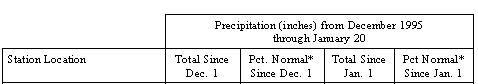
 Table 1.2 Precipitation data for December 1, 1995 through January 20, 1996
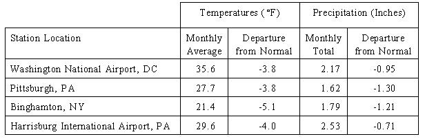
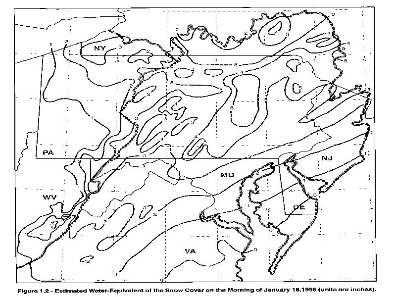
 Snow Cover A prolonged period of cold weather settled across the central and northern portions of the region in early December 1995 (Table 1.1). This allowed snowfalls from a series of storms to accumulate into an impressive snowpack. The majority of the snowpack that was in place at the onset of the flooding was from three separate snowstorms during the period of January 6-13. The biggest single contributor was the "Blizzard of '96," which occurred from January 6-8. Record amounts of snow were measured at many locations along the metropolitan corridor between Washington, DC, and Boston, Massachusetts, with accumulations of 2-3 feet common. Snow fell as far west as Kentucky and Tennessee and as far south as Alabama and Georgia. Record snow depths were recorded in Boston, Massachusetts; Harrisburg, Williamsport, and Philadelphia, Pennsylvania; and Bluefield, West Virginia. Following the "Blizzard of '96," an Alberta Clipper swept across the northern part of the region on Wednesday, January 10, depositing 4-10 inches of new snow across parts of western and central New York, 2-5 inches across the Baltimore-Washington corridor, and 1-3 inches across western Pennsylvania and West Virginia. The third storm of the week took a track similar to the blizzard, but was much weaker. Nevertheless, amounts in excess of 6 inches were measured from inland portions of the mid- Atlantic States northeast into interior New England, with 2- to 3-inch amounts more common along the coast. As a result of this succession of snowstorms, there was a significant and widespread snowpack in place across much of the area by Thursday, January 18. Figure 1.1 represents snow depths from all available National Weather Service (NWS) reporting stations on the morning of January 18. Snow depths of 2-3 feet were common from across western Maryland, central Pennsylvania, upper New Jersey, and into New York State. From southern Pennsylvania, across Maryland and West Virginia, and into Virginia, snow depths averaged 6-12 inches, with significantly higher amounts in the mountains. Figure 1.2 represents an estimate of the water-equivalent of the snow cover over the area on the morning of Thursday, January 18. Water-equivalents ranged from 0 inches in the far southeastern portion of the area to over 5 inches in areas from south central Pennsylvania to the Catskill Mountains of New York. The map represents the general trend in values and not the small scale variations that may exist in any individual watershed. The dominate type of snow data available in this part of the United States are snow depths. There were also some water-equivalent data available. In the OHRFC area there were water-equivalent readings from a number of coop stations. There were also some water equivalent measurements from some synoptic stations in the area. The National Operational Hydrologic Remote Sensing Center (NOHRSC) measures water-equivalent from airborne natural gamma radiation surveys based on requests from the RFCs during times when there is significant snow. Airborne surveys were made over the OHRFC area from January 11-15. Since there was significant melt over the OHRFC area between these dates and January 18, the airborne data were only used in a subjective manner in preparing the water-equivalent map. Water-equivalent data were also available from the U.S. Army Corps of Engineers (COE) and the U.S. Geological Survey (USGS). The Baltimore District of the COE makes periodic multiple point surveys to determine the average water-equivalent above 14 of their projects in the Susquehanna and Potomac drainages. Measurements were available for January 16-17. Measurements made by the USGS were available for seven locations in the Delaware Basin, but since they were taken from January 10-12, which was prior to the last snow storm, they were smaller. At locations with both depth and water-equivalent values, snow density could be computed and used to convert other depth values into an estimate of water-equivalent. Snow density ranged from less than 0.20 in areas where the snow cover had not yet ripened, to slightly over 0.30 in western and southern areas where significant melt had occurred in previous days. Areal snow coverage, as determined from satellite observations by the NOHRSC, was used to determine areas in the southeastern part of the area that were not covered by snow at this time. The water-equivalent analysis shown in Figure 1.2 used topographic information to help extrapolate the available data. It was especially important to take terrain information into account along the divide between the OHRFC and MARFC areas.
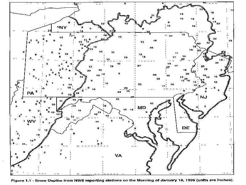
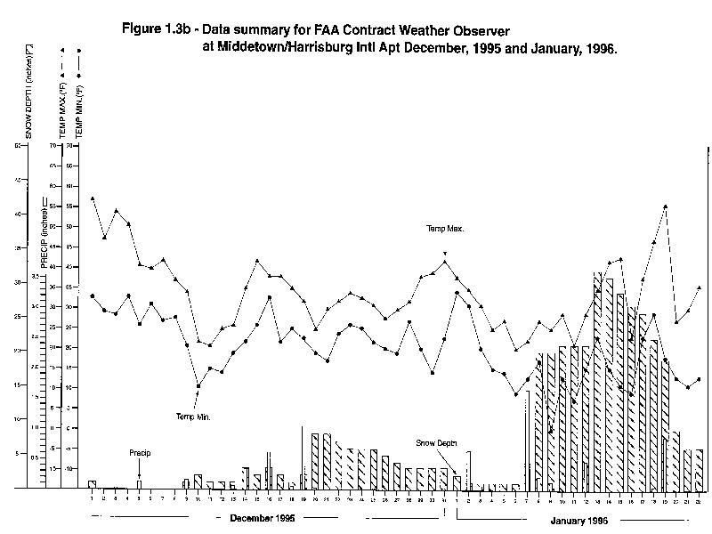
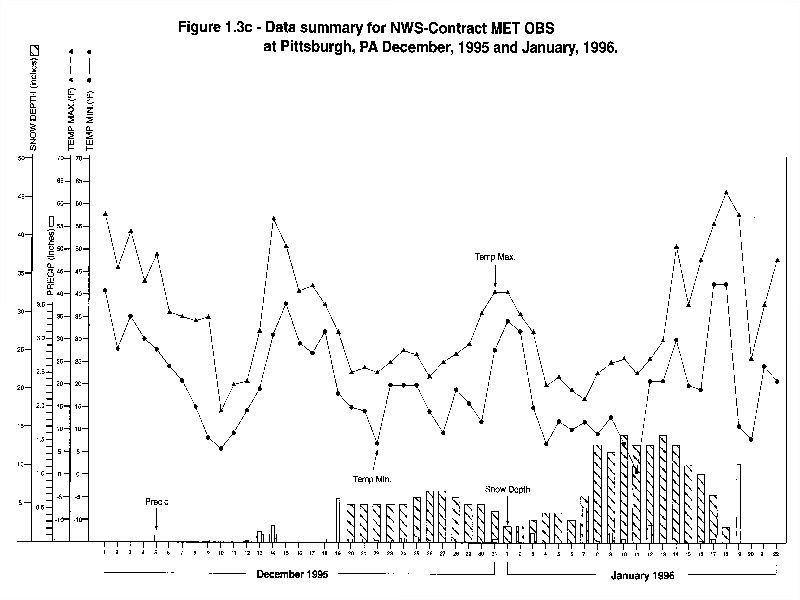
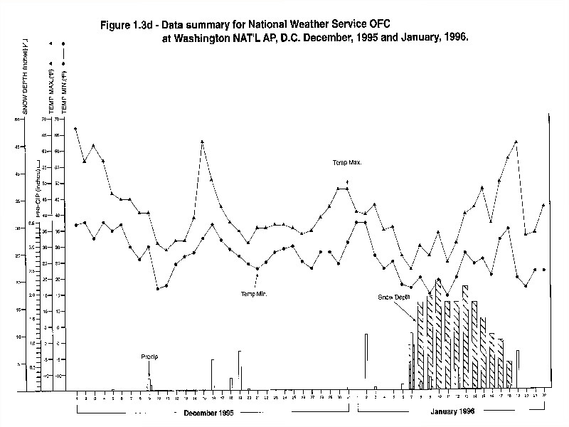
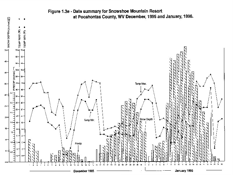
 Climatological Data for Selected Sites Figures 1.3a-1.3e represent the daily summaries for December and most of January of maximum/minimum temperatures, snow depth, and precipitation for Binghamton, New York; Harrisburg and Pittsburgh, Pennsylvania; Washington-National Airport in Washington DC; and Snowshoe Mountain Resort, Pocahontas County, West Virginia. The figures also show conditions during the event. These sites were chosen as representative of the antecedent conditions leading up to this flood event. Soil Moisture The soil moistures leading up to this event were normal for this time of year. Frost Depths Frost depths leading up to this event were minimal to nonexistent due to the extensive and deep snow cover insulating the ground during the colder weather preceding this event. River Ice River ice was common on rivers in northern Ohio, New York, Pennsylvania, New Jersey, and Maryland. Melting snow and ice break-up on the evening of Thursday, January 18, caused ice jam flooding across western portions of Pennsylvania and New York. Ice jams significantly added to the flood crests at numerous locations during this event.
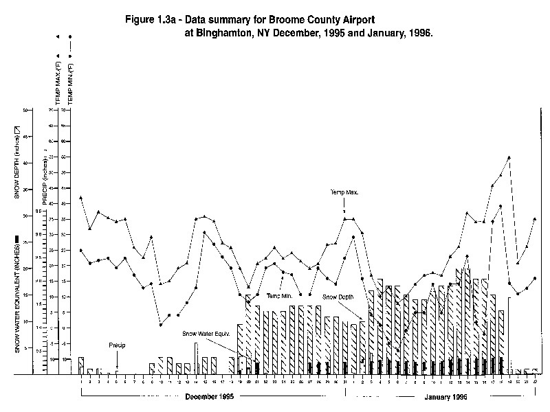
 Streamflow Prior to the flood event, streamflow throughout the region was generally characterized as a little below or near the long-term mean for January. Across central Pennsylvania, river levels were well below normal up until the thaw of January 18-19.
 1.3.2 HYDROLOGY Snowmelt The most unique aspect of this flood event was the intensity of the snowmelt. Not only was there an abnormally deep snow cover which covered a large portion of the area prior to the event, but the rate of snowmelt was extremely rapid. This is very unusual for this part of the United States. It is estimated that over the area of major flooding, about half of the available water came from snowmelt. The rapid snowmelt was caused primarily by the turbulent transfer of latent and sensible heat due to the high temperatures, dew points, and wind speeds. The major period of rapid snowmelt began in the western portion of the flood area on the morning of Thursday, January 18, and continued through the afternoon of Friday, January 19, in the eastern portion of the region. Generally, any given area experienced between 18-30 hours of high snowmelt rates. Figures 1.8a-d show calculated hourly snowmelt rates at four synoptic stations across the region. The figures show key data values and the breakdown of melt into the various energy exchange components. The snowmelt was computed using equations from Anderson (1976). Solar radiation, which was a minor factor during this period, was estimated from either percent sunshine (Hamon et al., 1954) or total sky cover (Thompson 1976), and the albedo of the snow surface was assumed to be 75 percent. Longwave radiation exchange was computed by taking the difference between incoming longwave radiation, calculated from the air temperature along with an estimate of the emissivity of the atmosphere (Anderson and Baker, 1967), and the outgoing longwave radiation from the snow surface at 0° C. Latent and sensible heat exchange, which clearly dominated during this event, were computed using an empirical wind function with a coefficient of .002 mm·mb-1·km-1. This coefficient is for wind at a height of about 1 meter above the snow surface. The wind speed data were reduced to the 1 meter level by using a factor of 0.5 at all stations, even though there was some variation in anemometer heights. Rain melt, which was significant during hours with heavy rain, was computed by assuming that the temperature of the rain drops were equal to the wet-bulb temperature. Data values for each hour were obtained by averaging the synoptic observations at the beginning and end of the hour. The computed melt rates shown in Figures 1.8a-d should be referred to as potential melt rates since, at some of the stations, the snow was gone at the site well before the melt period was over. At those sites, with most snow at the beginning of the event, the computed melt rates agreed closely with the depletion of the snow cover. At Binghamton just over 3 inches of water equivalent was reported on the morning of January 18, and the snow was gone at the site about mid-morning on Friday, January 19, based on the melt calculations. Middleton (Harrisburg) was the only one of these synoptic sites that did not lose all of its snow cover during the event. The snow depth at Harrisburg dropped from 23 inches to 9 inches during the intense snowmelt period, which was consistent with the energy computations.
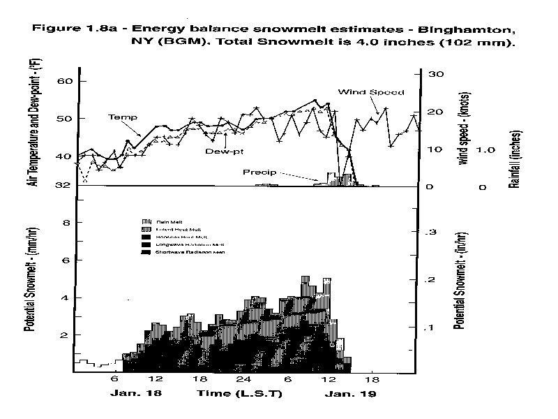
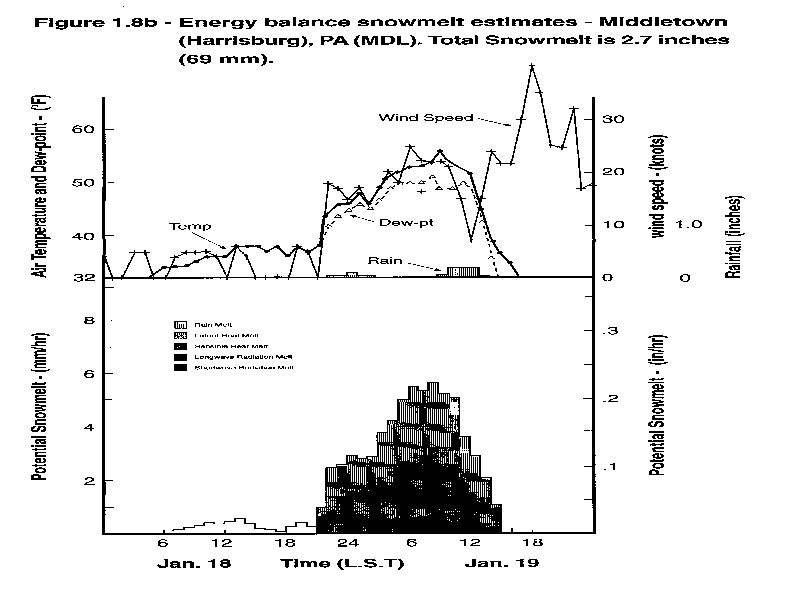
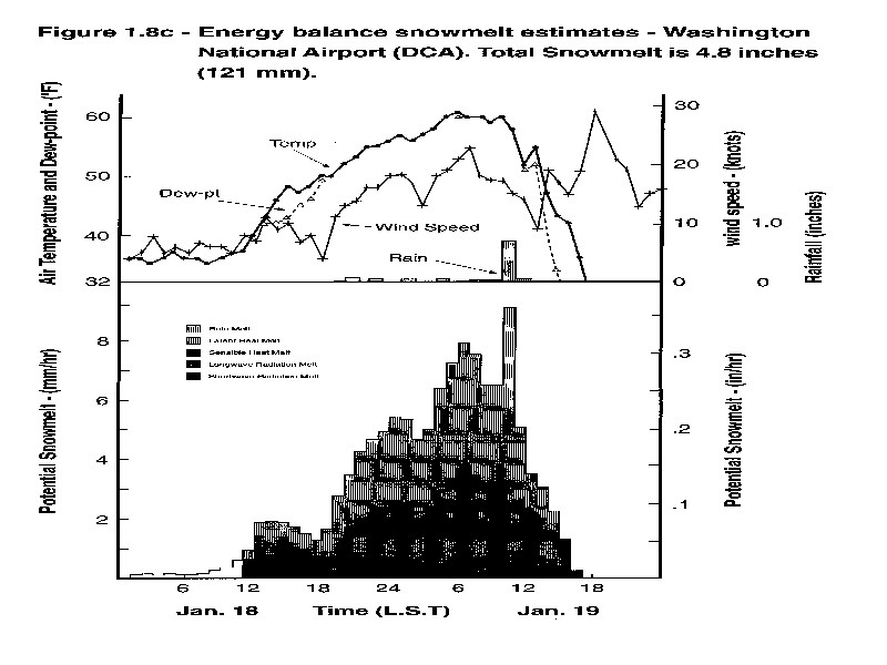
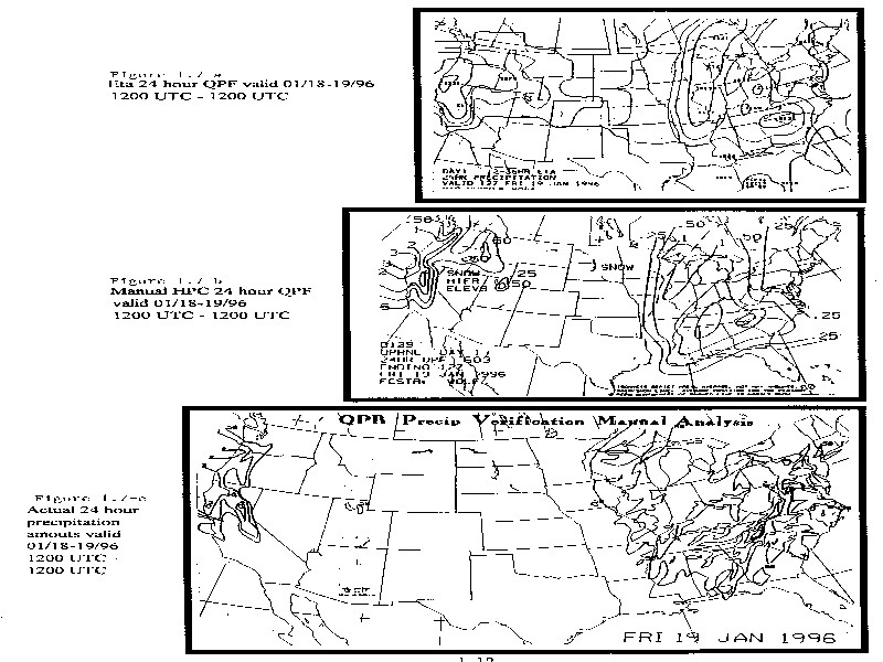
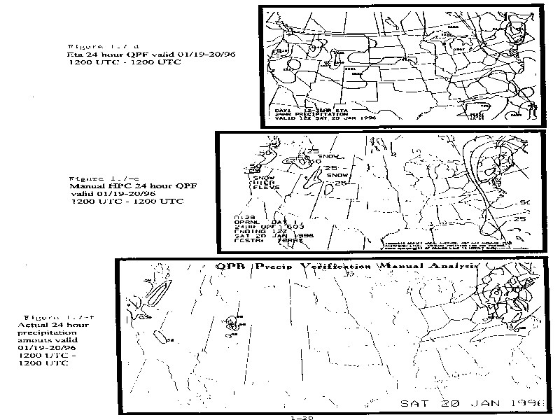
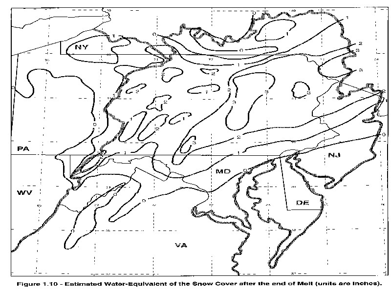
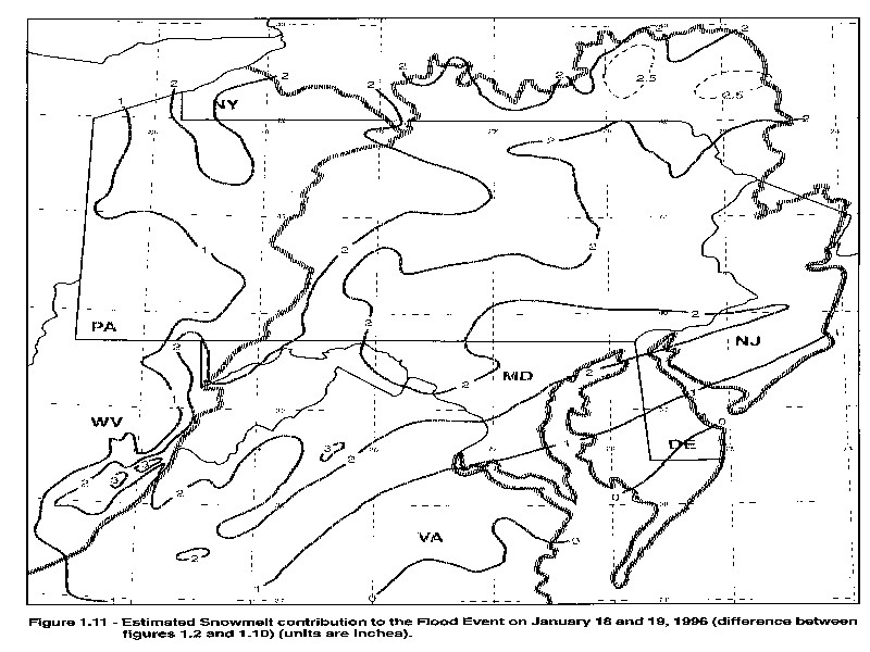
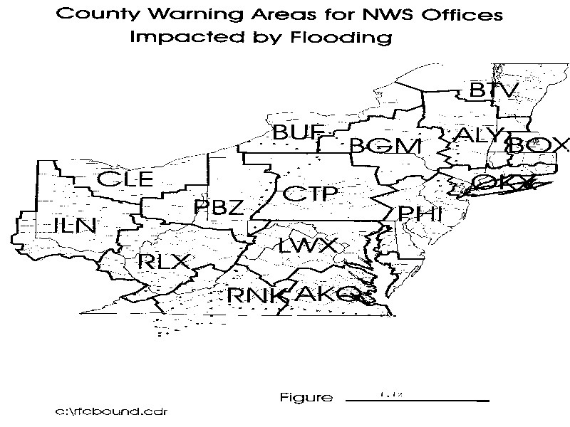
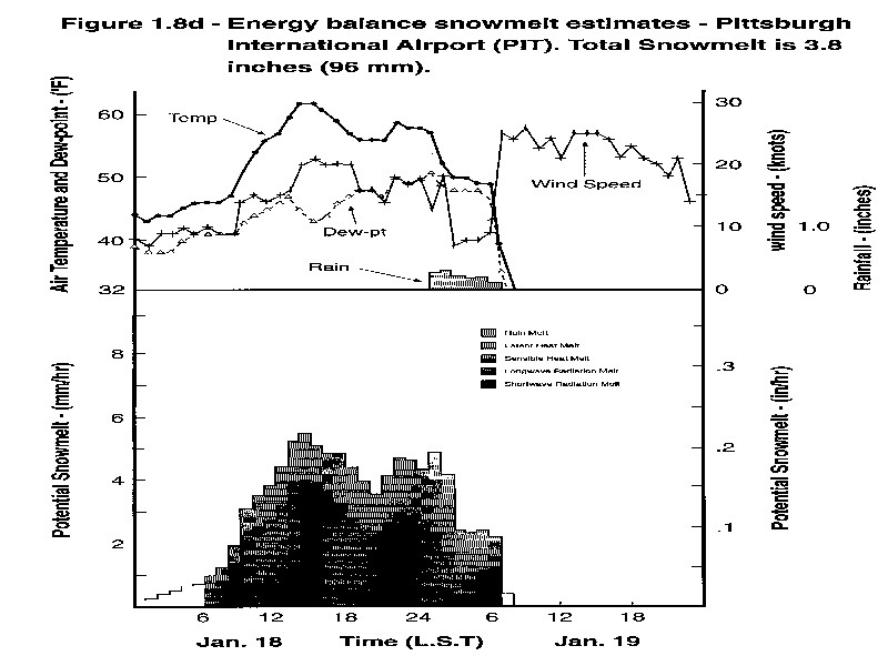 The energy budget computations of snowmelt indicated that at these synoptic stations the total potential melt ranged from just over 2.5 inches to nearly 5 inches during the flood period. These are computed melt rates for open, well exposed sites. Even for such a site, snowmelt rates of this magnitude are very rare, especially in the middle of the winter. For example, the maximum daily melt computed over a 7-year period at the National Oceanic and Atmospheric Administration (NOAA) snow research station in Vermont was 1.6 inches. This value occurred on a sunny day in late April. Snowmelt rates would clearly be less for the large portions of the area which were more sheltered from the gusty winds out of the south; however, the computations at these open sites help illustrate the mechanisms that caused the melt and give insights into the variation of melt rates over the region. Most of the area east of the divide between the OHRFC and the MARFC had a similar melt pattern consisting of low melt rates during the day on January 18, with a rapid increase in snowmelt late in the evening as the temperature, dew point, and especially the wind speed increased dramatically. The exception was in the northeastern part of the MARFC area, represented by Binghamton, where significant melt occurred throughout the afternoon and early evening of Thursday, January 18, due to moderate winds and temperatures and high humidity. West of the divide, there was also considerable snowmelt occurring throughout the day and into the evening on January 18, in addition to the high rates overnight. In order to get an estimate of the snowmelt contribution to the flood event over the entire region, consisting of forested and open areas over a variety of terrain, the amount of snow that remained after the flood event needed to be determined. Even with the very high melt rates that occurred during the event, there was still significant snow remaining over portions of the area. Figure 1.9 shows the snow depths reported to the RFCs on the morning of Saturday, January 20. Figure 1.10 depicts an estimate of the water-equivalent remaining after the flood event. As with Figure 1.2, the general trend is represented and not all the local variations. Local variations were accentuated by the time the event was over due to variations in melt rates resulting from small scale vegetation and terrain differences. Figure 1.10 uses data similar to those used to construct Figure 1.2. The relative geographical variation in melt rates depicted in Figures 1.8a-d were factored into the analysis as was topography. The snow remaining after the event was very ripe with densities around 0.3 or greater. It was recognized that many of the depth reporting stations were in exposed locations which would have less snow than the surrounding area after a significant melt period. Especially valuable in constructing Figure 1.10 were the data from the Baltimore District COE. A survey was made by the COE shortly after the event on January 22-23. The difference between the average watershed water-equivalents before and after the event were very useful and given significant weight in the analysis. Differences in water- equivalents over the area above the projects were generally in the range of 1.5-3 inches. The COE data also showed that, even in watersheds with considerable remaining snow, there were some bare areas. Runoff data from selected headwater locations were also used to estimate the areal average snowmelt contribution. The mean areal rainfall was subtracted from the total runoff (including an estimate of the increase in baseflow storage) to get an estimate of the snowmelt contribution. A local snow network maintained by the Binghamton weather office provided much detail on snow conditions in that area. Satellite observations from the NOHRSC were used to define areas with little or no snow cover. An effort was made not to include the light snow that occurred after the frontal passage on Friday, January 19, in the western and northern parts of the area. Figure 1.11 contains an estimate of the total snowmelt contribution to the flood event. This figure was constructed by computing the differences between Figure 1.10 and Figure 1.2. Figure 1.11 indicates that over the area of major flooding, snowmelt contributed from about 1.5 inches to over 2.5 inches of water. This is very similar to the amount of rainfall that was measured. In some parts of the area, the amount of available snow controlled the snowmelt contribution. This was especially true in most of the OHRFC area, much of Virginia, along the eastern edge of the region, and in portions of New York. Over the rest of the area, the snowmelt rates during the event determined the amount of available water from the snow cover. Figure 1.12 shows County Warning Areas (CWA) impacted by flooding. Rainfall By 8 p.m. EST on Thursday, January 18, rain had spread across most of Kentucky and Tennessee and was just entering southwest Ohio. Moderate to heavy rain was being reported in western Tennessee and Kentucky. In general, a 1- to 3-inch rainfall accompanied the cold front as it swept across the region on January 18-19. In some locations, six hourly amounts totaled between 2-3 inches. A record rainfall of 3.03 inches at Williamsport, Pennsylvania, broke the previous 24-hour precipitation record of 2.65 inches set in 1905. Total rainfall for the event, as reported by cooperative observers, generally ranged from 1-1.5 inches in east-central Ohio, and from 1.5-3.5 inches in Pennsylvania, New York, Maryland, and New Jersey. It is important to note that the majority of the rainfall in any one location typically fell within a 6- to 8-hour period. Orographic enhancement of the precipitation field also played a role in this flood event. A significant jump in the precipitation values occurred in the mountainous areas of the northeast United States. The observed rainfall for this event was significant in sections of the OHRFCs domain, as main-stem basins along the Upper Ohio River basin received average basin amounts exceeding 1 inch. For this same 48-hour period, the Allegheny Lower, Kanawha, and Monongahela Upper basins received basin average amounts exceeding 1.5 inches. Larger amounts of precipitation fell further to the east, within the umbrella of responsibility of the MARFC, as evidenced by MAP over the basin, exceeding 1.5 inches in 27 MAP areas within the MARFC. MAP for several of the basins in MARFCs forecast area exceeded 2.5 inches, and at least one basin exceeded 3 inches. It is important to remember that these heavy rains fell on a snowpack that was much above normal over the impacted area for this time of year. As the heavy rains fell on the ripened snowpack, it added to the rapid snowmelt that was occurring. The Upper Ohio River and mid-Atlantic drainage basins were quickly overwhelmed by the massive amount of runoff from the combined rain and snowmelt, resulting in major river flooding.
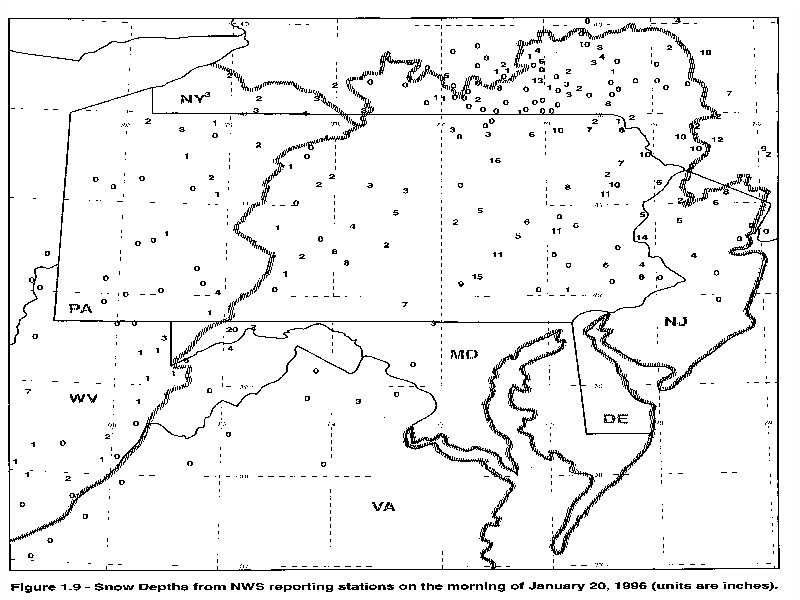
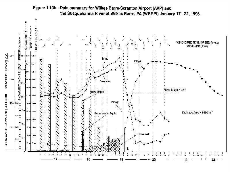
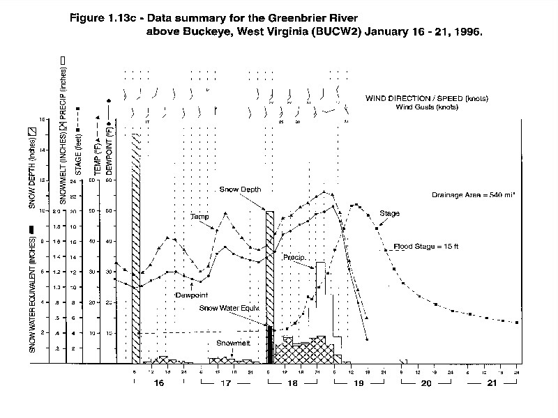
 River Response Hydrograph analysis for three key locations in the affected region (Figures 1.13a- 1.13c) showed that more than 50 percent of the observed runoff generated during this flood was from snowmelt in the 24- to 30-hour period prior to the onset of a 6-hour period of significant rain. Energy calculations indicate the potential for about 3-4 inches of water equivalent melt during the period. The snowmelt served to saturate the soils as well as provide 1-2 inches of surface runoff. The burst of rain associated with the cold front produced another 1-2 inches of runoff concentrated in a 6-hour period, whereas the snowmelt was spread over the 24- to 30-hour period. The runoff efficiency for the rainfall was quite high since soil moisture deficits had been well satisfied by the snowmelt, and thus a large portion of the rain converted to surface runoff. Snowmelt rates reached a maximum just as the rainstorm began, and the combination rain and snowmelt runoff was responsible for the sharp peaks in stage noted on headwater drainages. The snowmelt process was well underway for about 12-18 hours before a significant rise was noted on most of the flood prone rivers. The ripening of the snowpack, the satisfaction of soil moisture deficits, and surface detention storage were the hydrologic processes delaying the river response. Once the snowpack was ripened and the soils were primed, river stages rose quickly in response to the snowmelt runoff. Observers commented on the rapid rise in stage on even larger rivers, some saying it was "like a flash flood." The rapid rise observed was the direct result of the effects of ice jamming in the early part of this event and the fact that 100 percent of a drainage basin was contributing runoff. Prior to onset of the flood event, river discharges were in a baseflow regime. Cold weather during December and early January was of sufficient duration to develop a substantial ice cover on rivers in New York, Pennsylvania, New Jersey, Maryland, and northern Ohio. For ice jams to form, there must be a significant increase in river discharge before the river ice has a chance to weaken. This condition was well satisfied in this event. A progressive down-stream series of ice jams formed as the river ice cracked and separated into pieces resulting from the push of snowmelt runoff which lifted the ice and dragged it downstream. A low volume, high amplitude flood wave developed as a result of the release of ponded water from the failed ice jams. When a jam broke, the wave moved downstream to the next jam point resulting in a progressive downstream breakup front in which ice jams formed and released. When the breakup frontal wave passed a reach having a river gage, a rapid rise in stage was recorded, but because of the small volume of water entrained in the wave, the rise was short lived. If a large ice jam formed just downstream of a river gage, a rapid, and sometimes flood-producing rise would be noted. A more sustained rise from the runoff flood wave usually follows the breakup front.
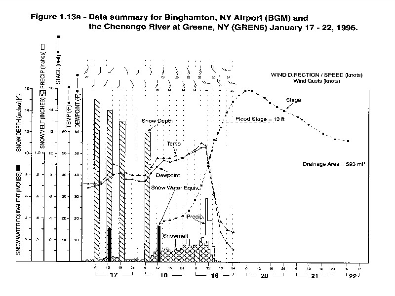
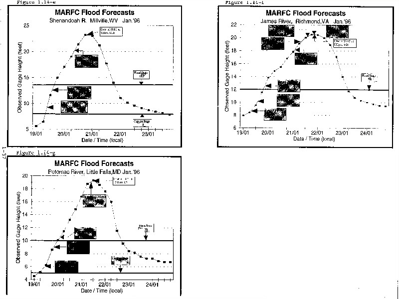
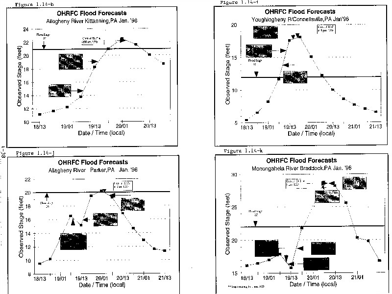
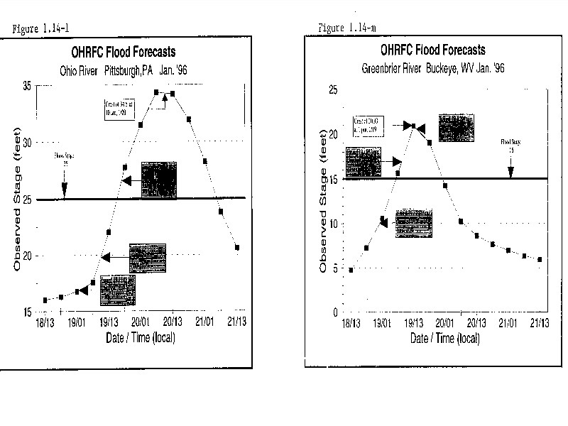
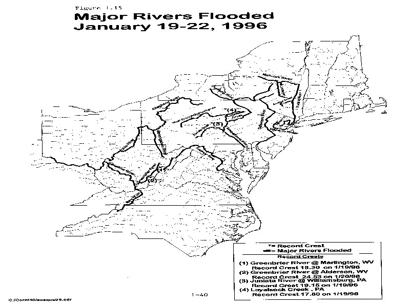
 A typical rain storm generates a relatively uneven space-time distribution of runoff on medium and larger drainage basins, whereas a snowmelt event, once the snowpack is ripened, will have a fairly uniform space-time distribution of runoff. Comparing a typical rainstorm with a snowmelt event, each having comparable intensities, durations, and antecedent conditions, the snowmelt events will have, on the average, the faster response times because of their more uniform and complete areal contribution of runoff. During the 30-hour snowmelt period, the calculated melt rates were on the order of 0.1-0.2 inches/hour which is the equivalent of moderate intensity rain. Coupling the nearly 100 percent areal extent of snow cover and the intensity/duration of the snowmelt, the generated streamflows from snowmelt alone were sufficient to send rivers at many of the affected locations above flood stage, particularly those draining the Appalachian highlands where snowpack was the heaviest. The rain merely added to the severity of the flood and increased the number of flooded locations. Overall rainfall and snowmelt runoff was by far the most important causal factor for this flood. The rapid drop in temperature behind the cold front halted the snowmelt and rainfall runoff process causing headwater streams to fall quickly back to within their banks in about a day, while larger rivers continued to convey the runoff for 3-4 more days before falling below flood stage. The magnitude of the flooding varied from basin to basin, but this was a major event. In Pennsylvania, both the Ohio River at Pittsburgh, and the Susquehanna River at Wilkes Barre, experienced their highest crests since Hurricane Agnes in 1972 (Pittsburgh crest affected by ice). The crest at Harrisburg was comparable to that observed with Hurricane Eloise in 1975. The Juniata River in Pennsylvania had a crest comparable to the flood of November 1950. The Delaware River at Trenton, New Jersey, had its highest crest since Hurricanes Connie and Diane in 1955. The south branch of the Potomac, Cheat River in West Virginia, and Monongahela River in Pennsylvania, reached levels not seen since the extreme Appalachian flood of 1985. The Hudson river at Albany, New York, crested higher than any time since 1977. Record floods were reported on Loyalsock Creek at Loyalsock, Pennsylvania; Frankstown Branch of the Juniata River at Williamsburg, Pennsylvania; Towanda Creek at Monroeton, Pennsylvania; Tunkhannock Creek at Dixon, Pennsylvania; Schoharie Creek at Burtonsville, New York; Beaver Kill Creek at Cooks Falls, New York; Delaware River at Callicoon, New York; Otselic River at Cincinnatus, New York; Willis Creek near Cumberland, Maryland; Opequon Creek near Martinsburg, West Virginia; and the Greenbrier River at Marlinton, West Virginia. Figures 1.14a to 1.14m are examples of hydrographs, including the NWS crest forecasts, for key locations in the OHRFC and the MARFC areas of responsibility. Figure 1.15 shows a map of all major rivers which flooded during this event.
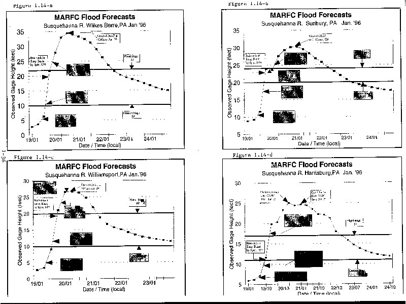
 The OHRFC has not calibrated the snow model to individual watersheds. Similar parameter values are used over the entire RFC area. These values are typical of a mostly open watershed with some forest cover. The RFC recognizes that these parameters tend to produce snowmelt that is more rapid than that observed in the eastern, forested part of their area during typical melt periods. The MARFC has calibrated the snow model to a number of individual watersheds over much of their area. They have used these results to regionalize model parameter values for many other watersheds.
  Both RFCs use event Antecedent Precipitation Index (API)-based models developed many years ago to compute the amount of storm runoff from rainfall plus snowmelt. Storm runoff is converted to discharge using a unit hydrograph and is added to baseflow discharge to generate the total hydrograph. In an event API model, the API value at the beginning of the event is used to compute an initial antecedent index, which is used along with accumulated storm rain+melt to compute accumulated runoff during the event. Between events the API value drops by a certain percent each day. After a few weeks with no rain or melt, this recession causes the API value to approach 0.0. After that it is difficult to determine the degree of dryness and its effect on runoff generation. During an extended period of snow accumulation there is no rain or melt, but the snow cover keeps the soil from drying out. In some API models, the API value is retained throughout a period with significant snow cover. This feature is an option in the OHRFC model, but is not used in the eastern portion of their area. The MARFC model does not use snow cover information to modify the API recession. The OHRFC API model uses one rainfall-runoff relationship for the entire RFC; however, temperature and latitude are built into the relationship so that there is some variability across their area. The MARFC API model uses a number of regional relationships to reflect the relationship between API and the antecedent moisture conditions. Evaluation One of the major challenges during this event, from the modeling standpoint, was determining the rate of snowmelt. As was pointed out earlier in this chapter, the snowmelt rate was abnormally high, especially for this time of year. The nonrain melt factors and the UADJ values needed for the SNOW-17 model to reproduce the melt computations shown in Figures 1.8a-d on a 6-hour basis were calculated. The results are shown in Table 1.4. For periods with slightly more than 0.05 inches of rain, both values are given. Typical melt factors for exposed locations, such as these, in mid- January are 0.6-1.0 mm·°C-1 · 6-hr-1. Typical UADJ values for such locations are 0.10- 0.13 mm·mb-1. As can be seen from the table, during the peak of the snowmelt the melt factors needed for this event are about 2-2.5 times greater than the typical values and the UADJ values are about twice as great as would normally be expected. It is also clear from this table that the adjustments needed to the melt rates need to be changing throughout the event as the meteorological conditions change. At the MARFC, the forecasters tried to use the nonrain melt factor correction in NWSRFS but found it difficult to determine reasonable values. The only information they had to look at was the computed and observed hydrographs which clearly contained other sources of error than just the rate of snowmelt. There was no method available to use meteorological data, in addition to temperature, to estimate the melt rate. Table 1.4 6-Hour Snowmelt Parameter Values Needed to Reproduce the Energy Balance Computations Shown in Figure 1.8.
 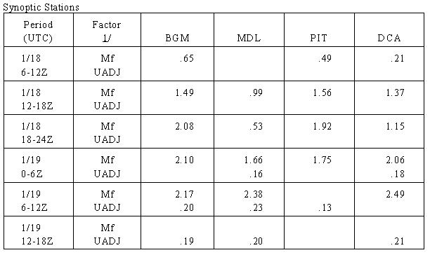 1/ Mf is the nonrain melt factor in mm·°Cܬ-hr-1, and UADJ is the rain-on-snowmelt parameter in mm·mb-1. The lack of such a method also prevented the RFC from using forecasts of dew points, wind speeds, etc., available before the event occurred, to generate a quantitative outlook that reflected the likelihood of abnormally high melt rates. In addition, even if methods were available to estimate the correction, the forecaster currently cannot easily determine what is happening inside the models so that they would know, for example, whether the nonrain or rain-on-snow equation is being used during a given time period.
 In addition to difficulties in determining the rate of snowmelt, other snow modeling- related issues evident from this event were the determination of the amount of water- equivalent prior to the start of melt and an understanding of the physics of a snow cover. The MARFC spends a lot of time monitoring the development of the snow cover. They carefully verify the modeled form of precipitation for each event and make corrections when necessary. The snow model water-equivalent values are also checked against available measurements; primarily COE project data and airborne snow surveys. It appears that this effort paid off as the RFC watershed estimates of water- equivalent prior to this event were very similar to those shown in Figure 1.2. The OHRFC relies primarily on the airborne snow survey estimates of water-equivalent provided by the NOHRSC to update the snow model initial states. For this event, the RFC updated water-equivalents for many of the runoff zones in the eastern part of their area on Tuesday, January 16, based on estimates provided by the NOHRSC. By the morning of Thursday, January 18, the RFC-modeled water equivalents were generally somewhat lower than the values shown in Figure 1.2 for the Kanawha and Monongahela drainages and similar for the Allegheny basin. Some of the differences were due to the updates and some due to the over computation of melt from January 16-18 caused by regionalized model parameters. For both RFCs, this effort would be much easier and lead to better overall results if an objective procedure was available to analyze all the snow observations as suggested by Recommendation 1.1. Prior to and after the event, there were comments from both RFCs that the snow cover would absorb a considerable amount of the forecasted rain and therefore the flood threat might not be as great as what actually resulted. At the MARFC, there was a "rule of thumb" that significant runoff from the snow cover would not occur until the density of the pack reached about 0.33. Thus, if the water-equivalent before the event was 4 inches and the depth 20 inches (initial density of 0.2), for example, the snow cover would hold 2.6 inches of water before reaching a density of 0.33. This type of thinking ignores the fact that if that much rain falls, the mechanical action of the rain will cause the snow grains to change and the depth will be considerably reduced, thus causing the pack to ripen and runoff to begin well before all the rain occurs. The overall knowledge of the energy exchange process may also not be as great as is necessary. Even though the SNOW-17 model only uses air temperature to compute snowmelt, it is important for users to understand the basics of the energy exchange components so that they may better anticipate when the model is likely to need adjustments.
  In addition to problems relating to snow accumulation and melt during this event, there also appeared to be a general underestimation of MAP, primarily in the mountainous portions of the region. There appeared to be a more pronounced than normal orographic component in the precipitation field for this event. This can be seen in Figure 1.12a. If there are enough functioning precipitation gages in an MAP area to represent all elevations and aspects, this does not present a problem. However, when there are only lower elevation gages, or the higher elevation gages are not operating, then the procedures currently used by the RFCs will provide an underestimation of the MAP values. The use of isohyetal analyses based on historical data to adjust station weights, as recommended for mountainous areas, would help correct the problem, but would still not handle the dynamics of the particular event. In order to make reasonable adjustments to the computed MAP values for a given event, the forecaster needs to be able to visualize how the precipitation is varying with the topography and how the variation compares with historical isohyetal values.
  The last modeling-related problem identified for this event involves the determination of the antecedent moisture conditions. The event API models used by both RFCs are developed based on data from storm events. The technique for computing the change in moisture conditions between events does not involve any evaporation or water balance calculations, but merely is based on reducing the API value by a certain percent (typically 10 percent) each day. The reduction in API is the same during a dry period in the summer, when evaporation rates are high, as during a period of snow accumulation during the winter. In the MARFC area, the API values had dropped to 0.1 (their allowable minimum) over the northern part of their area, as a result of nearly continuous snow cover, with very little melt during the 6-7 weeks prior to the event. In the OHRFC area, the API values were not generally this low because of melt that had occurred over a several-day period prior to the event. After the event, the MARFC made some runs for selected watersheds, comparing simulated discharges with an initial API of 0.1 versus an initial API of 1.0, which would be more typical of late January. These runs showed a 9-21 percent increase in peak flow with the wetter initial conditions.
  In recent years the Office of Hydrology (OH) of the NWS has begun to develop and implement an Advanced Hydrologic Prediction System (AHPS) that will be able to generate an ensemble of possible predictions so that the uncertainty of the forecast can be quantified. This quantification of uncertainty is based on the Ensemble Streamflow Prediction (ESP) procedure that is used at several RFCs. AHPS hopes to refine the estimates of uncertainty by taking into account factors such as weather forecasts, model error, and errors in initial state variables, in addition to future climatology as is currently done with ESP. Procedures like ESP are especially valuable when the current conditions, such as an abnormally large snowpack as in the case of this event, will have a major impact on what happens in the future. ESP and AHPS technology would have been an extremely valuable tool to have had available for this flood event. With such a tool, quantitative statements could have been made of the likelihood of various flood levels being exceeded. One factor, illustrated by this event, that needs to be considered when developing improvements to ESP is that model error (in this case the error in calculating snowmelt from air temperature alone) would have to be conditioned on the weather forecast (at least once the weather forecast could indicate that high dew points and wind speeds were likely). It should also be made clear that ESP and AHPS technology requires that the hydrologic models be properly calibrated in order to produce reliable answers.
|
Main Link Categories: Home | OHD | NWS |