by: Tom Bradshaw & Lara Bradshaw
I. Introduction
As we all know, the accurate forecasting of winter-time precipitation type is probably the most challenging task we face as meteorologists here in Alabama. Seemingly minor vertical variations in temperature and dew point can play a pivotal role in determining what falls out of the sky and onto area roads, trees, and power lines . Over the years, the forecasters at this office have gained considerable experience observing relationships between various thermodynamic fields and precipitation types. However, it's probably safe to say that none of us has precisely isolated all of the possible correlations that may exist between these parameters and the occurrence of snow, sleet, and freezing rain. Even if we could adequately corner these relationships, another formidable challenge would lie in assessing the degree to which the models are accurately depicting these fields in time and space.
The articles through the years devoted to winter weather - and the forecasting of it - could easily be used to paper a trail from the Herrmann/Wells Smoking Area to the balloon shelter - and back. The determination of precipitation type alone has been addressed by a crowd of authors over the past half century, including several who have focused exclusively on the problem as it relates to the Southeast United States. However, few have attacked the topic to the extent that Samuel Contorno treated it in his 1992 Master's Thesis at the University of Oklahoma. A wealth of valuable, Alabama-specific information is contained in this document, information we can exploit to produce improved forecasts for our area.
Fundamentally, all weather predictions, in one way or the other, are probabalistic. Overtly or not, we assign a degree of confidence to each element we are forecasting. For example, if the models are predicting a winter precipitation event, then we may have to consider the possibility that freezing rain, sleet, or snow may occur. The confidence we assign to our forecast of precipitation type will depend on many factors, chief among them:
a) the models' projection of temperature, and/or thickness at the time of the event, and the degree to which these parameter values correlate to that precipitation-type's long-term climatological frequency of occurrence, and
b) the degree to which we believe the models' accuracy in predicting these parameters.
Regarding the former, there is much that can be gained by considering long-term frequency distributions of precipitation-type vs. the basic parameters of temperature and thickness. Analyses of this type are at the heart of Samuel Contorno's study. As for b), a host of other studies must be undertaken to assess the error characteristics of the various models' thermal fields. Such an investigation is beyond the scope of Contorno's work.
Unfortunately, to date we haven't made full use of Contorno's findings, simply because they haven't been all that accessible to the forecasters on staff. This poster represents an attempt to rectify this problem. What follows are a series of scanned duplications of Contorno's key figures, plus a number of excerpts from his thesis. It should be emphasized that most of the following text has been taken directly from Contorno's thesis; brackets [ ] have been used to distinguish between Contorno's writing and our own.
II. Methodology
Contorno examined all precipitation events which occurred in north Alabama between November, 1974 and December, 1988, with the goal of assembling an appropriate sample of cases for each precipitation type. As part of his study, he obtained hourly surface observations from the Birmingham airport (BHM), as well as daily RAOB soundings from Centreville (CKL). Prior to 1974, rawinsondes were released from Montgomery, which is too far from Birmingham for one to draw relationships concerning sounding parameters and precipitation type.
Contorno established several criteria for including a precipitation event in his study:
Using these criteria, Contorno obtained 63 events, 4 of which were removed for use as an independent sample to validate the results of his decision tree. The following is the breakdown of occurrences of each precipitation type:
| Precipitation Type | Nbr. of Occurrences |
|---|---|
| Rain | 21 |
| Frzg rain/drzl | 8 |
| Ice Pellets | 10 |
| Snow | 20 |
| Total | 59 |
It's interesting to look at the breakdown of precipitation types listed above. Over the 14 year period of the study (and at surface temperatures of 36 deg F or colder), snow events were just as likely to occur as rain events were. Moreover, snowfalls were twice as frequent as freezing rain or sleet events were. Though derived from a short period of studyt, the occurrence frequencies listed above should be factored into a forecaster's decision-making process when he/she is considering the possibility of a snow, freezing rain, or sleet event.
II. Physics
As part of his study, Contorno discussed some of the important microphysics related to the formation of frozen precipitation. Cutting to the chase, here are two of the big points to remember:
III. Sounding Variables used in Study
In his thesis, Contorno presented frequency distributions relating precipitation type to a variety of different thermodynamic parameters. The following graphics depict each of these frequency distributions, while short excerpts from his thesis are used to discuss these parameters.
1. Variable 1: Coldest T in a saturated layer below 500 mb and above the boundary layer
[Variable 1 helps to determine whether cloud layers exist at cold enough temperatures to activate ice nuclei. If saturated layers exist with temperatures below -4 deg C, it is possible that ice formation can occur; for higher temperatures, it is very unlikely. This is a very effective variable in separating out freezing drizzle cases, which might occur when the entire sounding is below freezing, from snow or ice pellet cases.]
[The histogram demonstrates the expected relationship between snowfall and the maximum temperature at which ice nuclei takes place (approximately -4 deg C). No snow event occurred when Variable 1 was above this maximum value. The same holds true for ice pellet cases which also require ice nuclei activation to exist. The maximum occurrence for snow and ice pellet events was in the -10 to -20 deg C range which coincides with the temperature range where ice crystal growth by vapor deposition is at a maximum.]
2. Variables 2 through 7: Wet bulb temperatures at various layers
[Variables 2-7 take into account the effects of evaporational cooling on precipitation type in various layers by using the wet bulb temperature. An individual snowflake or rain droplet actually experiences a temperature very near the wet bulb temperature as it falls due to evaporational cooling in sub-saturated air. Because of this, ice may be able to survive above freezing temperatures if the wet bulb temperature is low enough, and largely melted ice particles may be able to refreeeze for the same reason. Wet bulb areas are calculated by taking the layer means of wet bulb temperature at 10 mb increments, and weighting them with respect to the natural log of pressure.]
3. Variable 8: Mean temperature of the surface to 1000 m layer
[Variable 8, the mean temperature of the surface to 1000 m layer, represents the approximate average temperature of the boundary layer. This variable is useful in that it helps to determine the amount of melting or freezing which might be occurring close to the ground.]
[All but two snow events had a value below freezing. Meanwhile, all but two of the ice pellet cases had values above freezing. Since many ice pellet cases occurred with average wet bulb temperature layers below freezing, this would indicate a dry low-level environment with strong evaporational cooling.]
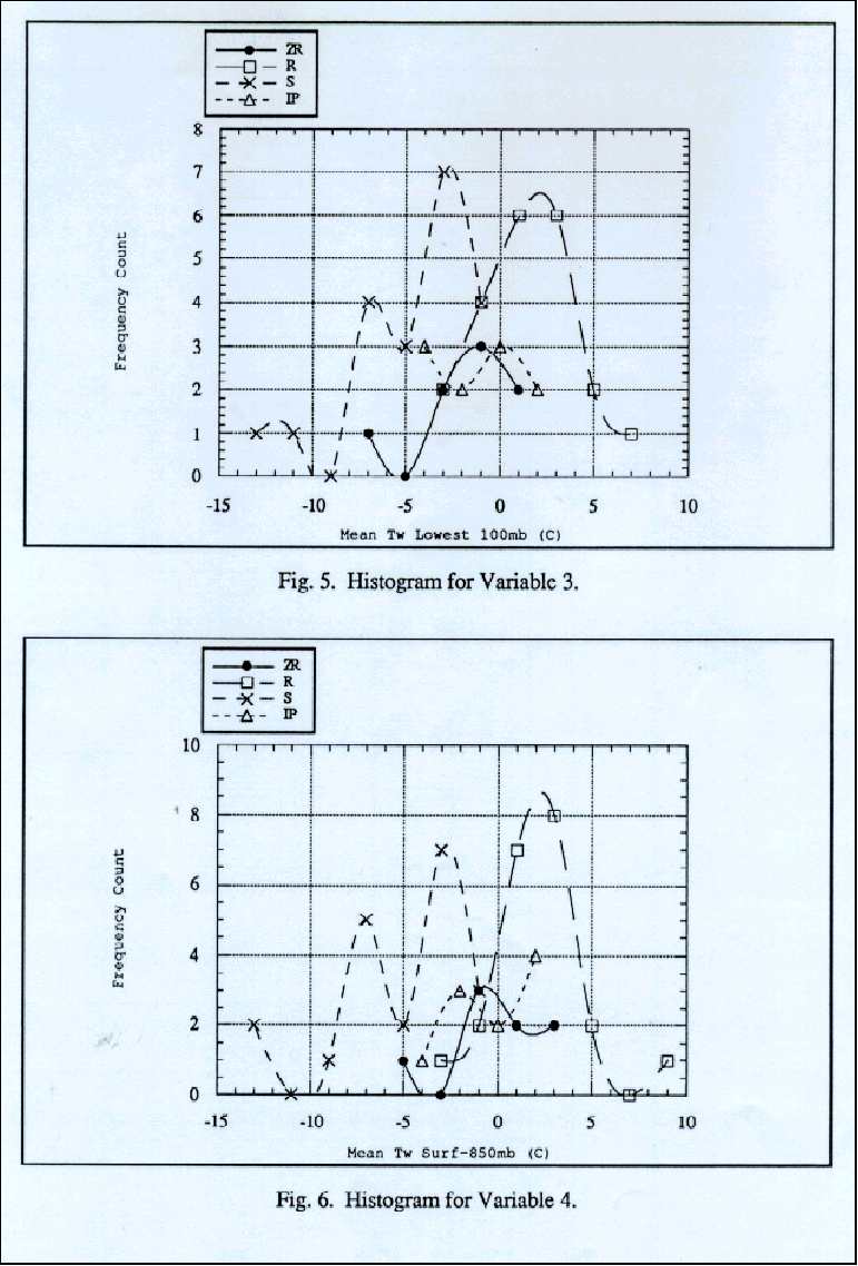
4. Variables 9 and 10: Surface values of temperature and wet bulb temperature
[Variables 9 and 10, the surface values of temperature and wet bulb temperature, are straightforward but useful. The surface temperature is the main variable which separates freezing rain/drizzle cases from rain cases. Since both of these habits reach the ground in liquid form, the surface temperature determines whether a droplet will freeze on contact. A better predictor would be the actual ground temperature since it is possible that very warm/cold conditions prior to the precipitation episode would allow/not allow droplets to freeze despite above freezing/sub- freezing temperatures. The surface wet bulb temperature gives insight to the evaporational cooling that might occur at that level.]
[The histogram for this variable demonstrates the best predictor between rain and freezing rain/drizzle cases. Five freezing rain/drizzle cases fell in the 0 deg C bin, the maximum value recorded for that precipitation type, while all but one rain case occurred with temperatures above freezing. Snow and ice pellet cases fell over a larger range of temperatures; therefore, this variable is not an effective predictor for these precipitation types.]
[The histogram for the mean surface wet bulb temperature, indicates that snow events possessed the coldest surface wet bulbs on average, but surprisingly, eight events occurred with above freezing values, falling in the 2 deg wide bin centered at 1 deg C. Ice pellet cases ranged from -4 to 4 deg C. Two rain cases happened with values below freezing, but the vast majority of events occurred with wet bulb temperatures above freezing, with the mode at the 1 deg C bin. All but one freezing rain/drizzle case fell with surface wet bulb temperatures below freezing.]
5. Variables 11 through 14: 1000-700 mb thickness, 1000-850 mb thickness, 850-700 mb thickness, and 1000-500 mb thickness
[Variables 11-14 are the classical thickness values of various layers which have long been used in precipitation-type forecasting. Thicknesses are directly proportional to the mean virtual temperature in the layer under question. Therefore, lower thickness values may indicate a likelihood for ice formation or survival while higher values may indicate a likelihood for liquid precipitation. It is important to remember that thicknessess represent average temperatures for the entire layer. It is possible that warm or cold regions may exist within the layer which might melt or freeze falling precipitation without significantly affecting the overall thickness value. Because of this, specific values of thicknesses cannot be related to a specific type of precipitation with full confidence.]
[The histograms for the four thickness variables prove that these variables can be useful predictors. The maximum bin value for snow in the 1000-700 mb distribution is 2850 m. Only one freezing rain/drizzle and one ice pellet case occurred with a value less than that. The complicating factor is that three rain cases also occurred within the 2850 m bin. Despite these cases, 87% of non-snow events occurred with 1000-700 mb thicknesses above 2850 m.]
[The 1000-850 mb thickness histogram indicates another sharp snow cut-off value. All snow cases occurred with values less than 1307 m (within or below the 1300 m bin). Nearly 80% of non- snow cases occurred with 1000-850 mb thickness values of greater than 1300 m. The histogram for the 850-700 mb thickness does not reveal as sharp a cut-off value between snow and non- snow events. Four snow and eleven rain cases coincided with the 1550 m bin.]
[Meanwhile, the 1000-500 mb thickness histogram gives an excellent discrimination between liquid and ice cases. No liquid precipitation event occurred with a thickness value less than 5400 m! In fact, only one non-snow event occurred with a value less than 5400 m (an ice pellet case). The 5400 m thickness value has long been used as a rain/snow line; for north-central Alabama, this appears to be reasonable. It should be noted, however, that snow and ice pellet cases did occur with 1000- 500 mb thicknesses greater than 5400 m. For snow, the maximum was 5471.5 m; for ice pellets, it was 5551.0 m. In general, although good at distinguishing between snow and non-snow cases, the thickness variables do little to distinguish between rain, freezing rain/drizzle, and ice pellet cases.]
6. Variable 15: Surface-based area below 850 mb where Tw < 0 deg C (Deg m); Variable 16: Area of sounding below expected ice nucleation level where Tw > 0 deg C (Deg m)
[Variables 15 and 16 are "area"quantities which are calculated by taking the product of the depth of a layer and the mean wet bulb temperature in that layer. Therefore, these variables have units of Deg m.]
[Variable 15 is the surface-based area below 850 mb where the wet bulb temperature is less than 0 deg C. The quantity is set to zero if the surface wet bulb temperature is greater than 0 deg C. For larger values of Variable 15, it is more likely that evaporational cooling will allow ice to fall through the lowest layers of the atmosphere unmelted or that partially melted particles will refreeze. The lowest part of the atmosphere was emphasized in deriving this variable to point out the unexpected snow or ice pellet occurrences when surface temperatures are warm, yet evaporational cooling allows for the survival of ice particles.]
[Variable 16 is the sum of all areas below expected ice nucleation level where the wet bulb temperature is greater than 0 deg C. This quantity points out melting layers in the sounding. Any warm layers (temperatures > 0 deg C) above the highest expected ice nucleation level (temperature <= -4 deg C and dew point depressions = 2 deg C) are omitted since these layers would have no effect on the melting of ice particles.]
[The histogram for the area of the sounding below the expected ice nucleation level where the wet bulb temperature is greater than 0 deg C proves that this variable is a useful predictor. Of the rain cases, only the anomalously cold event produced a value of 0 Deg m. The next lowest value rose to 504.9 Deg m, while the rest of the values ranged to a maximum of 20251.0 Deg m. All freezing rain/drizzle cases had values greater than 757.6 Deg m, revealing the warm inversion above the surface which melted falling ice particles. Ice pellet cases showed a similar range as that of the freezing rain/drizzle cases. The snow cases were omitted from this histogram. The reason for this omission is that the maximum value for this variable was only 318.8 Deg m. In fact, the next highest value was only 88.1 Deg m. Therefore, these small values could not be accurately displayed with the 2000 Deg m bin size employed for the other precipitation types. The fairly wide range between the maximum snow value and the minima for the other precipitation types makes Variable 16 an excellent precipitation-type predictor.]
8. Variable 17: Net area of sounding below 850 mb with respect to 0 deg C wet bulb temperature
[Variable 17 is the net area below 850 mb with respect to 0 deg C wet bulb temperature. A positive value of this variable indicates net regions of wet bulb temperatures above 0 deg C and the potential for melting. A negative value indicates net regions of wet bulb temperatures below 0 deg C and the potential for freezing. Variable 17, unlike Variable 15, is not set to zero if the surface wet bulb temperature is above freezing. The advantage of using a "net area" predictor is that it considers melting and freezing layers together, giving an overall effect. Warm layers may exist, but if they evenly co-exist with cold layers, an ice particle may still reach the ground.]
[The histogram for the net area below 850 mb with respect to 0 deg C wet bulb temperatures, reveals improvement on information given by Variable 15. All snow events yielded negative net areas. Seventeen out of 21 rain cases had positive areas. In general, the ice pellet and freezing rain/drizzle cases have similar traces on the graph, with some positive and negative net area events. However, ice pellet cases had a lower mean value (-788.0 Deg m compared to -325.5 Deg m for freezing rain/drizzle cases). From this information, it can be interpreted that the average ice pellet event, as compared to a freezing rain or drizzle event, may experience regions of slightly colder wet bulb temperatures, allowing for the preservation of the ice state.]
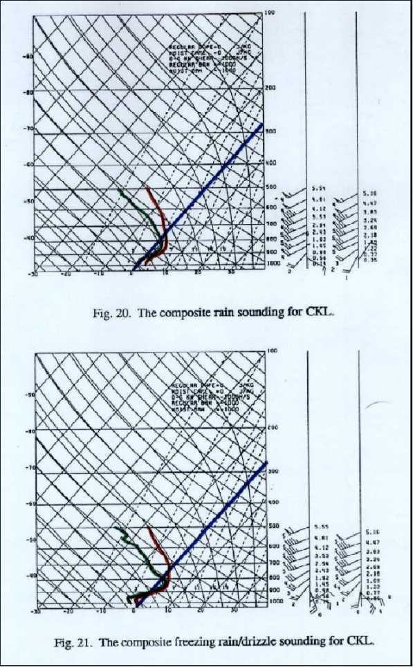
IV. Composite Soundings for each Precipitation Type
In addition to the histograms, Contorno used data from the 59 cases to produce composite soundings for each precipitation type. Without further ado, here they are (red line is temperature, green line is dew point, and blue line is 0 deg C isotherm):
[The rain composite indicates a sounding entirely above freezing up to approximately 750 mb. Except for a very small region around 950 mb, the dew points are also above freezing, leaving little question that any ice particles falling through this part of the sounding would melt. Low-level veering of the winds indicates warm air advection with the rain events.]
[The freezing rain/drizzle composite reveals the expected sounding structure for this precipitation type. A nearly 100 mb thick sub-freezing layer extends upward from the surface, and it gives way to an inversion which has a maximum temperature value of about 3 deg C at 850 mb. The air wihtin the inversion is nearly saturated; therefore, no significant evaporational cooling could take place to preserve ice particles. Any ice that might fall through this inversion would melt but freeze on contact with the sub-freezing ground. As with the rain composite, veering low-level winds indicates a warm air advection pattern.]
[The snow composite indicates sub-freezing temperatures throughout the sounding. The lowest dew point depressions are found between the surface and 800 mb, but no layer is as moist as some seen in the freezing rain composite. In general, the snow soundings contained more variability than the freezing rain soundings. For example, soundings taken just before the onset of snow often exhibited significant dry layers near the surface. Other soundings were almost saturated throughout the lowest layers. Because of this, the average of these sounding types tended to "wash out" saturated layers. The snow composite indicates northwesterly surface winds veering in the lowest 100 mb but backing through a deeper layer in the mid levels. This pattern points out low-level warm air advection and mid-level cold air advection.]
[The ice pellet sounding composite shows a dry layer (dew point depressions approximately 5 deg C) from the surface to about 850 mb. Above that, a region of moister air (dew point depressions approximately 2 deg C) exists. Despite above freezing temperatures up to 750 mb, the wet bulb temperatures remain near 0 deg C due to the large dew point depressions. The wind patterns are remarkably similar to those seen in the freezing rain/drizzle composite.]
V. "Warm Sleet" Considerations
[In the course of the study, ice pellet events with surface temperatures well above freezing (one as high as 44 deg F) were encountered. The sounding structure of these events differed significantly from the composite ice pellet sounding for the Oklahoma City area. It was hypothesized that the precipitation processes in the "warm sleet" CKL soundings were quite different from the "classical" ice pellet soundings. The hypothesis states that ice particles form in saturated and sub-freezing regions of the soundings, fall through other sub-freezing saturated regions where growth by riming occurs, and enters the warm surface layer. Since the surface layers are very dry on average, low values of wet bulb temperature allow ice particles to reach the surface in ice form as highly-rimed snow pellets or graupel particles.] For additional information on "warm sleet" processes, please refer to copies of Contorno's chapter on this topic which have been placed on the training clipboard, and in the Public Forecaster Handbook, located next to the Public Forecaster's Desk.
A link to a section discussing warm sleet will be added here in the near-future.
VI. Construction of a Decision Tree for Forecasting Precipitation Type
After compiling the frequency distributions shown above, Contorno used several of the discriminators derived from them to construct a precipitation-type decision tree. Basically, the first component of the tree involves a test to determine if the coldest temperature in a saturated layer is less than -4 deg C, which is the minimum value required for ice nuclei activation. If it is not, then frozen precipitation particles cannot form - only liquid ones can. At this point, it is left to determine if the precipitation will be freezing rain, or just rain. The test for this determination is the temperature at the surface; if it is less than 0 deg C, then freezing rain will occur.
If the minimum saturated layer temperature is less than -4 deg C, any of the four precipitation types could exist. One could then employ 1000-500 mb thickness to discriminate between liquid or freezing precipitation and snow, since none of the former types occur with thickness values below 5400 m. The remainder of the flow chart involving the sleet/freezing rain cases gets a bit complicated, but it basically involves a combination of Variables 16, 17 and surface temperature.
VII. Final Thoughts
As we've just seen, the Contorno study provides us with a wealth of information concerning the relationships between sounding variables and winter precipitation type. Briefly, here are some of the main points again:
Microphysical Considerations:
Thickness Considerations:
- The peak frequency for snow cases was 1280-1300 m (min = 1258 m; max = 1307 m)
- The peak frequency for freezing rain was 1320 m (min = 1278 m; max = 1344 m)
- The peak frequency for ice pellets was 1310 m (min = 1298 m; max = 1354 m)
Other key thermodynamic variables:
Variable 16 (the sum of all areas below expected ice nucleation level where the wet bulb temperature is greater than 0 deg C) is a good discriminator between snow and ice pellets. All snow cases occurred with values of Variable 16 less than 350 Deg m. On the other hand, all ice pellet cases occurred with values greater than 725 Deg m.
While Contorno's findings are important, the question of their operational employment is just as critical. While the Contorno decision tree can be utilized with observed soundings, it is obviously preferable to apply it to hourly model soundings, given the latter's lead time and high temporal resolution. BUFKIT, with its ability to display wet bulb temperature, is an excellent source for much of the thermodynamic data required by the decision tree. However, an accurate determination of Contorno's "wet bulb areas" by visual means alone is not easy. Hopefully, the authors of BUFKIT can be convinced to modify their software to display these special parameters.
In the meantime, a simple local program (called "Snowtree") will shortly be available to process sounding data and render a proposed precipitation type using Contorno's decision tree. Snowtree requires temperatures and dewpoints at several levels between the surface and 500 mb in order to calculate the needed parameters. Unfortunately, at the present time these data have to be manually typed into the program, and this is a slow, time-consuming process. In addition, Snowtree doesn't utilize as many different model layers as a more sophisticated software package like BUFKIT might. This results in cruder, more error-prone wet-bulb area calculations. However, it is currently the only way to derive the special wet bulb parameters needed by Contorno's scheme. In the near-future, a slightly modified version of the Snowtree program will be placed on the PC's in the Operations Area. This version will allow you select the number of model levels you wish to enter into the program.
Finally, an important factor to consider when forecasting precipitation-type is the degree of potential error in the the models' thermal fields. In particular, a knowledge of the long-term bias characteristics of the models' temperature, dewpoint, and thickness fields can be extremely useful when assigning confidence to a winter precipitation forecast 24 to 48 hours hence. For example, if the ETA is forecasting precipitation with a 1000-850 mb thickness of 1302 m, it would be helpful to know what percentage of the time the model accurately predicts thickness values within this range, versus the frequency with which it is too warm or too cold. To partially answer this question, a small study has been undertaken to evaluate the error characteristics of the ETA's thickness and 850 mb temperature fields during the winter and spring of 1996-1997. Findings from this study will soon be available as a link from this page.


 Follow us on YouTube