by Richard V. Thacker
Senior Forecaster - WFO Charleston, SC
In a spring season with several unusually intense convective events across the southeast states, severe thunderstorms struck the Palmetto State on May 10th, producing a rare strong tornado near the city of Charleston. The bulk of the damage, rated as a strong F2 [ Fujita and Pearson, 1973] by a team of storm investigators from NWSO Charleston, occurred in Dorchester County in the vicinity of Summerville. In the Main Street, Market Area, and Sangaree Subdivision, 5 homes were destroyed and at least 25 other homes suffered some structural damage. Unfortunately, the tornado caused 1 fatality and 10 people suffered injuries.
On May 9th, 1998 the upper air pattern across the contiguous United States was fairly typical of mid May in regards to the existence of several cut-off low pressure systems. One aspect of the pattern was the presence of a rather strong low latitude jet stream which extended from the southwest states to the southeast coast. This southern stream feature had been a trademark of the spring season to date, possibly related to the existence of much warmer than normal water temperatures in the Pacific Ocean. Earlier in the spring, a 175 knot jet streak helped evacuate rising air in the upper levels over Alabama spawning an extremely rare F5 tornado in the Southeast United States which nearly destroyed the town of Oak Grove, just west of Birmingham.
The 500 mb pattern at 0000 (all times UTC) Sunday May 10th indicated a broad but progressive short wave near the Kansas/Oklahoma border with a trough that extended southward over Eastern Texas. An impressive jet maxima at the 500 mb level ranging from 75-95 knots was observed across northern Mississippi, Alabama, and Georgia (FIG 1). At 850 mb at 0000, a low height center was located over Arkansas. A band of 15o C dew points and 30-40 knot winds stretched from west of New Orleans, LA to Jackson, Mississippi and northwest to Memphis, Tennessee and Little Rock, Arkansas (FIG 2). Weak ridging was occurring over Georgia and South Carolina in the mid and upper levels.
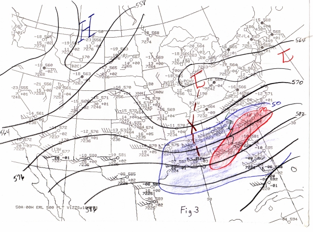
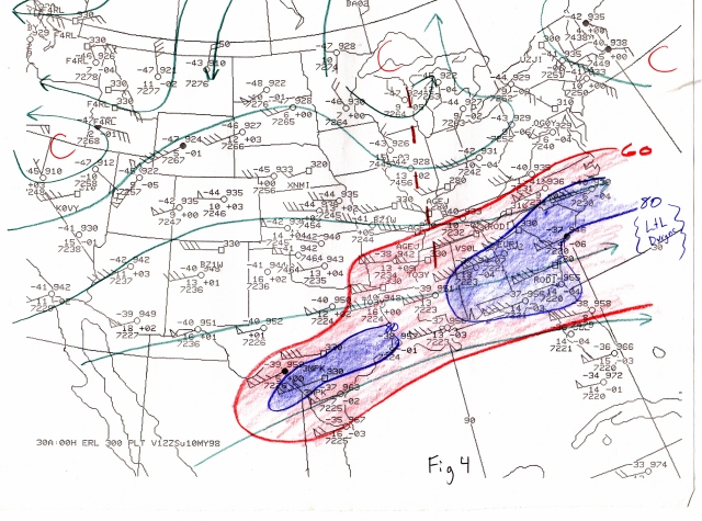
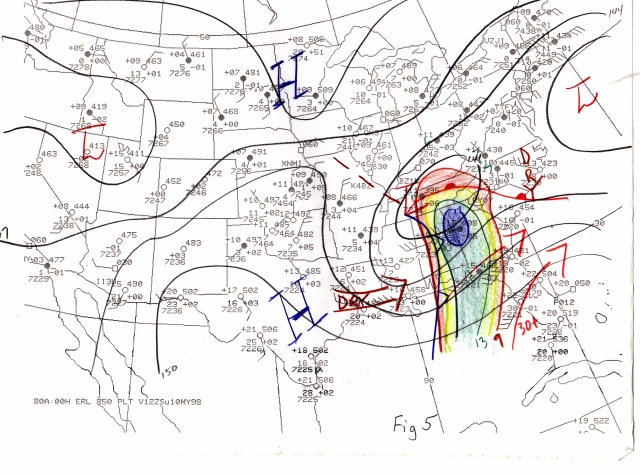
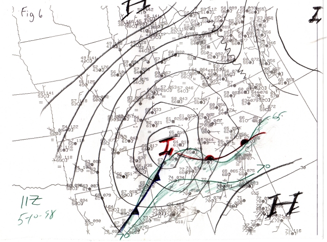
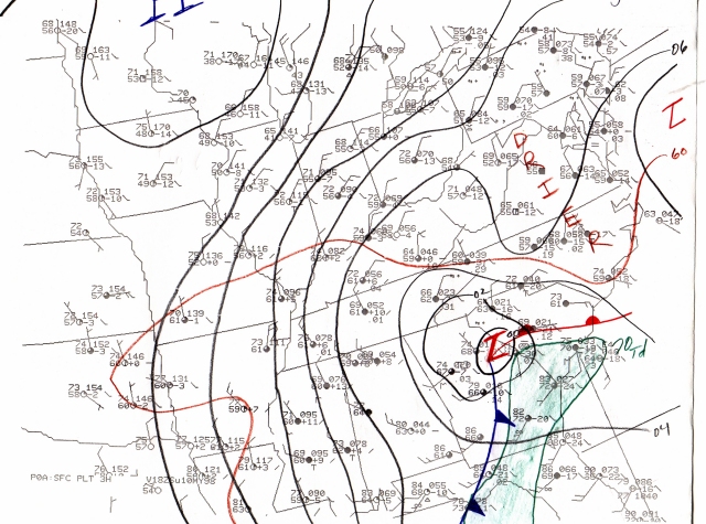
On May 10th at 1200, the 500 mb trough had progressed eastward and slightly de-amplified from western Tennessee south to southern Mississippi (FIG 3). The core of the mid level jet maxima stretched from the Florida panhandle northeast across southern Georgia into eastern South Carolina. At 300 mb, a jet core of 80 to 90 knots was over the southeast United States (FIG 4). At 850 mb, a warm front extended from central Tennessee southeast through the north coast of South Carolina. In the warm sector, impressive theta-e advection was occurring over Georgia poised to spread over much of South Carolina during the day. West to southwest winds at 850 mb in the warm sector were in the 30 to 40 knot range (FIG 5). The surface analysis at 1100 indicated a low pressure area over northern Alabama with a warm front extending from central Georgia to near Charleston. Dew points in the warm sector were in the upper 60s to around 70o F while north of the warm front, surface dew points were in the upper 50s to lower 60s (FIG 6).
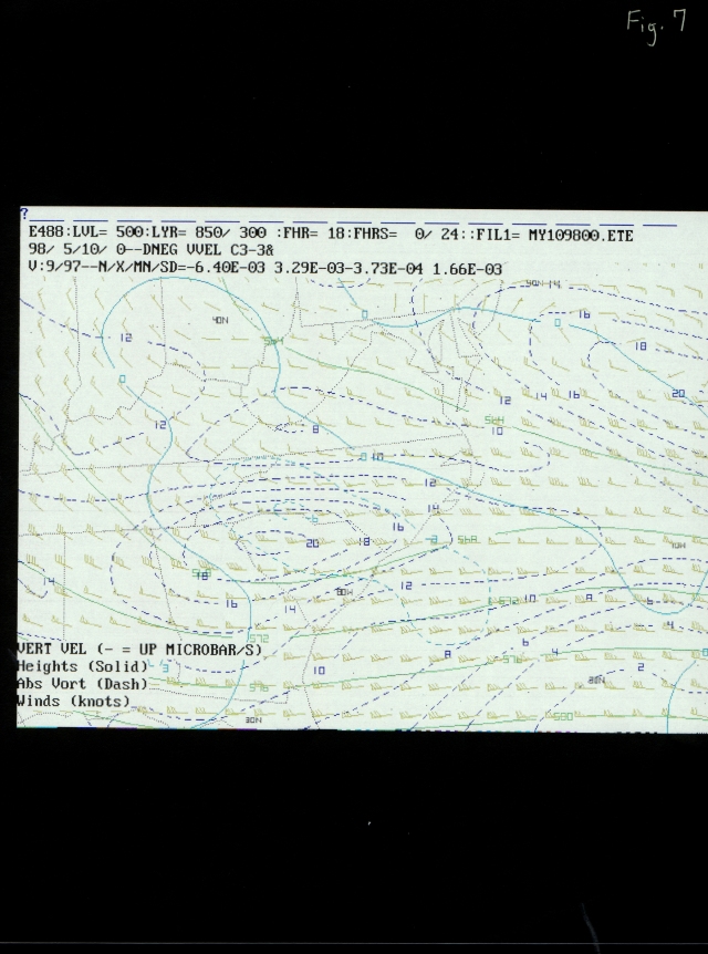
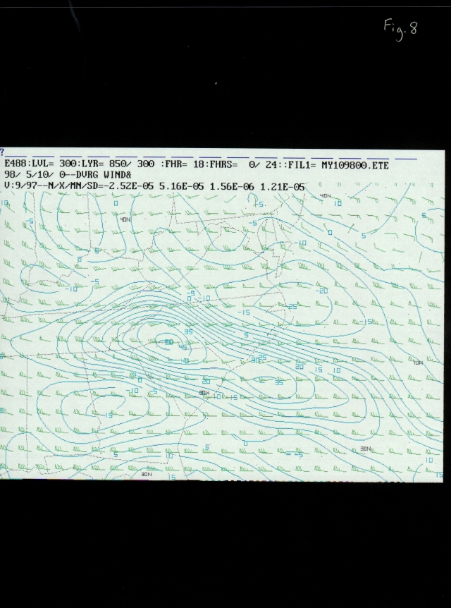
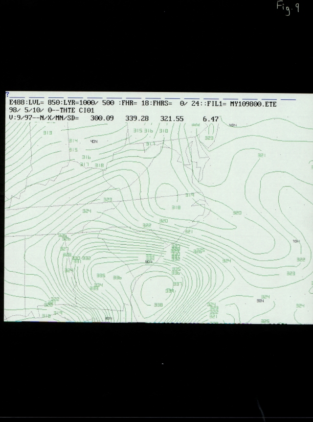
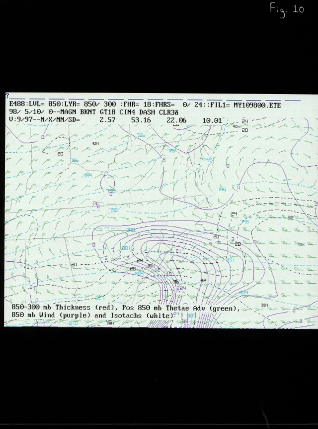
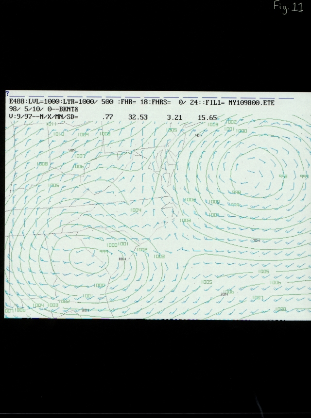
Using the initial 24 hours of the ETA output from 0000 May 10th, it was clearly evident that mid and upper level dynamics combined with a strong warm frontal boundary in the lower levels would lead to convective development along and south of the surface warm front once thermodynamics improved during the day. Forecast products valid at 1800 May 10th, showed the 500 mb short wave passing through western South Carolina with a 20 unit vorticity maxima (FIG 7). Divergence aloft at 300 mb was forecast to maximize across South Carolina during the same time frame (FIG 8). At 850 mb, a theta-e maxima was forecast just off the south coast of South Carolina with a extremely tight gradient from Charleston to Wilmington North Carolina (FIG 9), strong wind speed convergence was forecast along coastal South Carolina in unison with a ridge of theta-e advection. Broadly difluent thickness was noted in this same general region (FIG 10). On the surface, the low pressure area was forecast to be near the Augusta, Georgia vicinity at 1800 (FIG 11) while strong surface moisture convergence was forecast to extend from Augusta to Charleston (FIG 12).
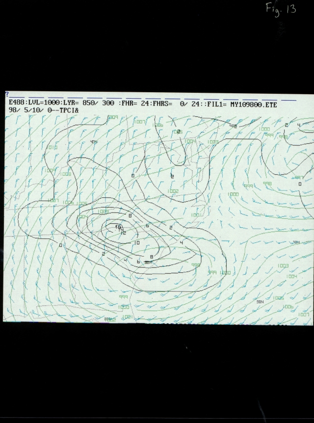
The ETA forecast output at 0000 May 11th, indicated the surface low pressure would move offshore of the South Carolina coast with lingering moisture convergence near Savannah, Georgia and Beaufort, South Carolina. The 12 hour forecast QPF showed a maxima extending from Greenville, South Carolina to Columbia and Charleston (FIG 13). In this short review of only ETA guidance, 2 things stand out: the warm front would enhance local helicity and the favored region encompassing tight moisture and stability gradients would be in close proximity to the surface warm front.
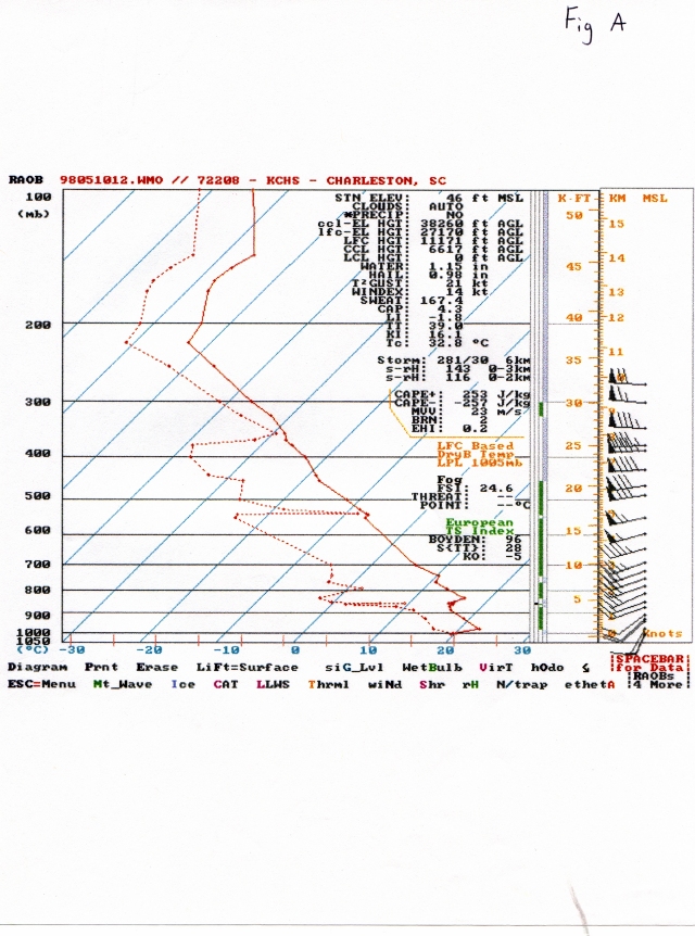
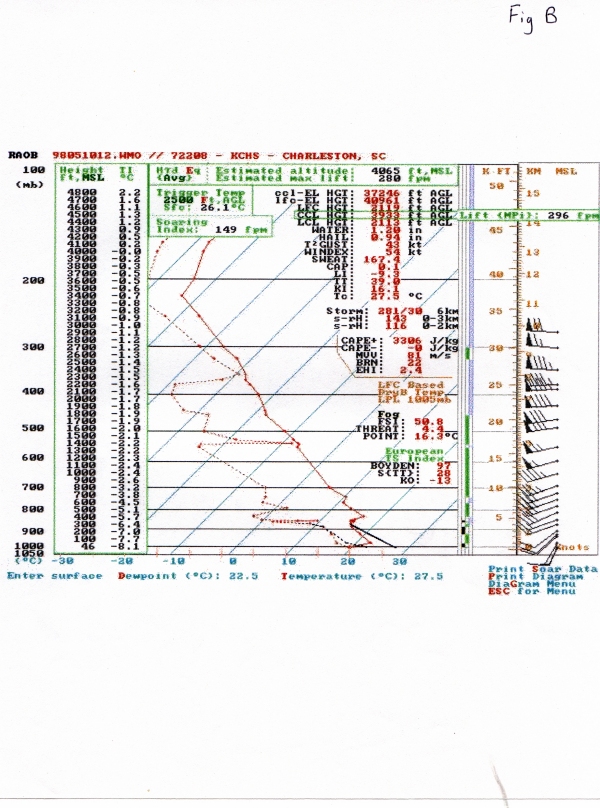
The May 10th 1200 sounding from Charleston indicated a marginally unstable atmosphere along coastal South Carolina but a rather dry column of air overall. Wind fields surface to 700 mb veered with height although speeds were relatively light (FIG A). After modifying the sounding using a surface temperature of 27o C and 22o C dew point, the atmosphere showed much greater instability. The modified CAPE was 3300 j/kg and the lifted index was -9 (FIG B). Upper air analysis indicated moisture advection at all levels would be occurring during the day.
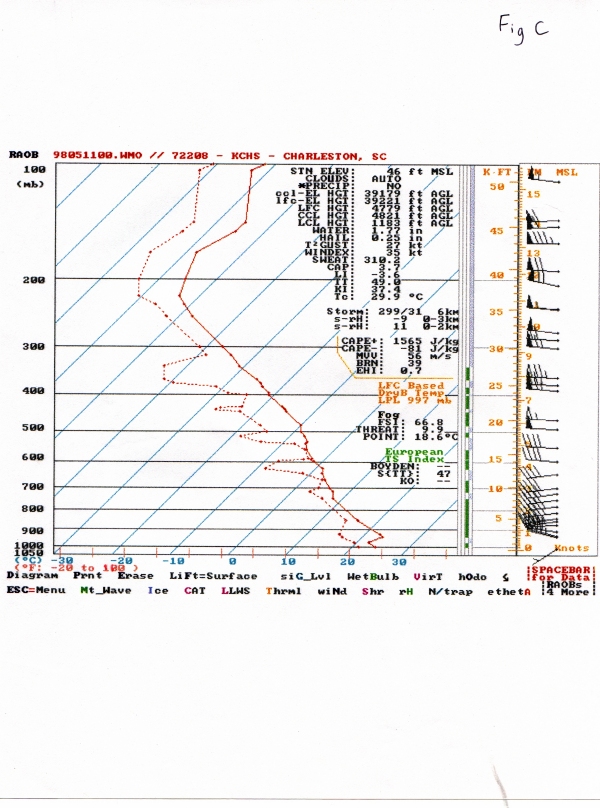
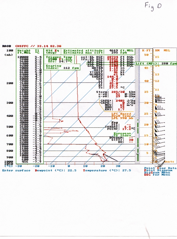
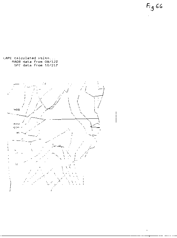
Inspection of the May 11th 0000 sounding revealed that the column had become more saturated. The K index had risen from 16 at 1200 to 37 at 0000. Other parameters such as the total totals index and precipitable water has also increased (FIG C). To give a perspective of a possible real-time storm environment, an experimental modified sounding was generated halfway between Charleston and Atlanta, Georgia using the RAOB PC software application (FIG D). This product revealed a steeper lapse rate but was unable to detect the presence of the moisture transport above 700 mb which was evident on the 0000 Charleston sounding. This experimental sounding modified with a surface temperature and dew point of 27o and 22o C respectively, did indicate a greater WINDEX value (61 knots) and forecast hail size (1.22 inch) than either of the observed or modified Charleston soundings. This greater parcel buoyancy was likely advected across eastern South Carolina during the afternoon.
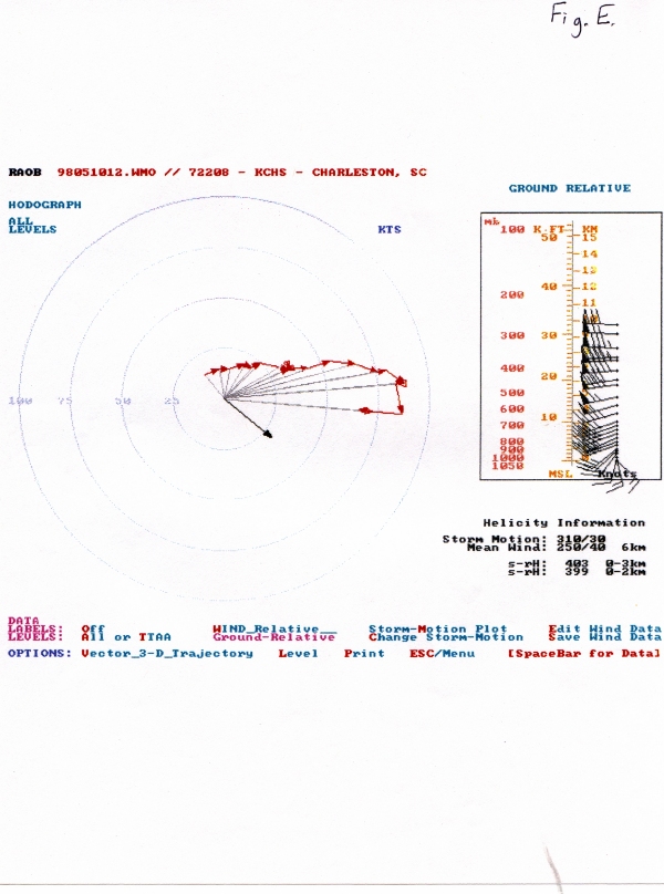
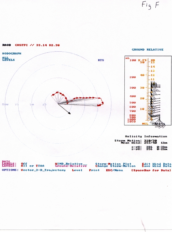
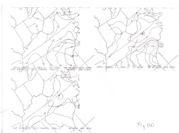
The prime interest in the pre-storm environment was the available low level speed and directional shear available for the formation of tornadoes. Since the warm frontal boundary became more enhanced across coastal South Carolina during the afternoon hours on May 10th, low level backing of the mean flow was not evident on the 1200 Charleston sounding. The analyzed 25-35 knot 900-700 mb wind field across Georgia was used to modify the 1200 Charleston hodograph which yielded a helicity value of approximately 400 in the first 3 km. Visual appearance of the hodograph gave the forecaster a hint of straight line multi-cell thunderstorms rather than tornadic supercells despite impressive boundary layer directional shear (Fig E). The modified experimental sounding from halfway between Charleston and Atlanta with identical low level wind fields, showed greater directional shear in the boundary layer with a helicity value of approximately 390 in the first 3 km (Fig F). The direct presence of the surface warm frontal boundary was obviously a major key in increasing the low level directional shear as witnessed by these modified hodographs and the surface analyses presented in the next section.
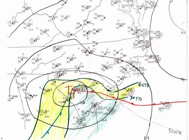
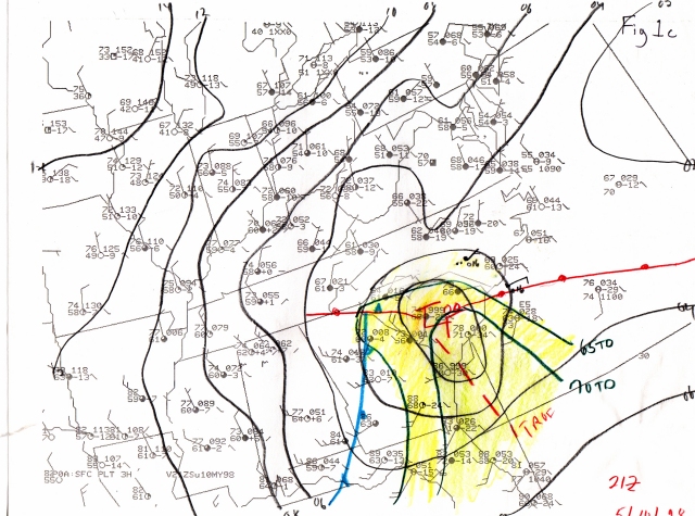
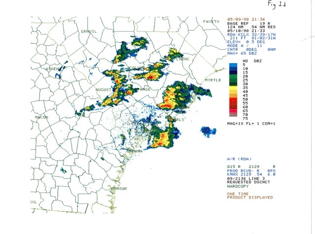
The first occurrence of severe weather in the Charleston County Warning Area on May 10th was in Screven County, Georgia where a small tornado touched down in the town of Sylvania at 1845. The brunt of the activity occurred in Dorchester and Berkeley Counties in coastal South Carolina between 2100 and 2200 (Fig 1a). A sequence of hand-plotted surface analyses shows a 1000 mb surface low moving almost due east from near Augusta at 1800 to Columbia by 2100 (Figs 1a-1b-1c). The warm frontal boundary was nearly stationary from near Georgetown, South Carolina west to the low pressure center. The warm sector encompassed the southern half of South Carolina with surface temperatures in the upper 70s to low 80s while north of the warm front, temperatures were in the mid 70s and dew points were only around 60o. The low was extremely well defined with strong convergence clearly evident looking at the surface plots.
From the NWP discussion, difluent flow aloft was spreading across the region in tandem with increasing positive vorticity advection in the mid levels. The dynamics aloft were maintaining the organized surface system and linking with improving thermodynamics in the warm sector leading to rapidly developing convection along and south of the warm frontal boundary. Further west between Augusta and Columbia, convection was aligned in a cyclonic fashion in the vicinity of the surface low pressure center and directly underneath the mid level vorticity maxima (Fig 1d).
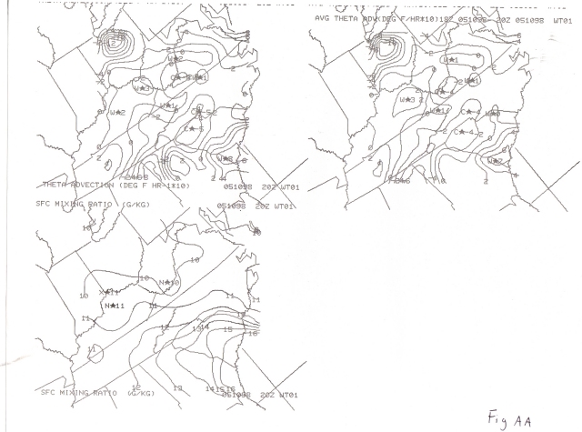
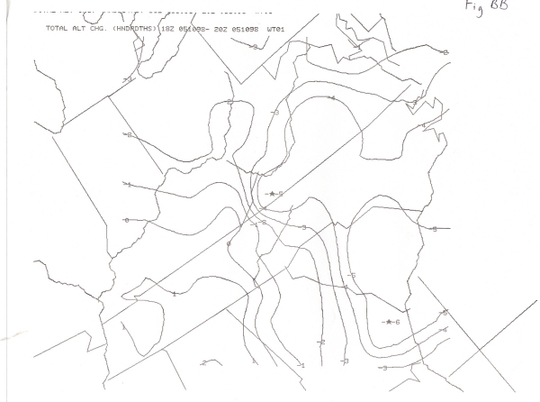
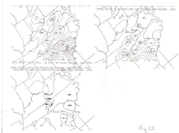
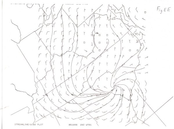
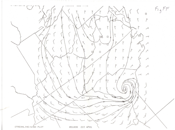
ADAP distinctly showed the gradient of both instability and moisture transport across the central coastal areas of South Carolina between 1800 and 2000. Theta advection was maximized over southern South Carolina in the heart of the warm sector. The Charleston area was in the tightest theta gradient and also on the warm side gradient of surface mixing ratios (Fig AA). Rather significant pressure falls were occurring from 1800 to 2100 ahead of the surface low, however a clearly defined rise-fall couplet was not evident. This was likely due to the fact that convection was just developing in unison with the maximum time of diurnal pressure falls (FIG BB). Clearly the surface moisture convergence was impressive by examining the surface analysis and ADAP clearly showed tremendous convergence across nearly the entire state, with the greatest convergence in the vicinity of the well defined surface low (Fig CC). A sharp gradient of surface-base lifted indices was also in place across the north central South Carolina coast with values ranging from -10 near Beaufort to -2 at Myrtle Beach (FIG DD). Surface streamline analysis indicated the low pressure area was becoming even better defined as it moved eastward just south of Columbia from 2000 to 2200 (FIG EE and FIG FF).
PC-CAPE indicated a ridge of 1500-2000 j/kg from Beaufort north to Columbia. It is important to note that Charleston was once again in the tightest gradient region (FIG GG). The gradients were all associated with the clear definition of the warm frontal boundary and while these gradients proved a breeding ground for convection, the sharp increase in speed and directional shear added a strong local helicity gradient as well.
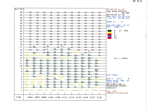
One would expect the Vad Wind Profile from KCLX to have shown a defined low level backing of the wind field near the time of the tornado on the ground within 20 miles of the station, however it is important to note that the radar site is located in Northern Jasper County or approximately 45 miles southwest of the developing tornado in Dorchester County.
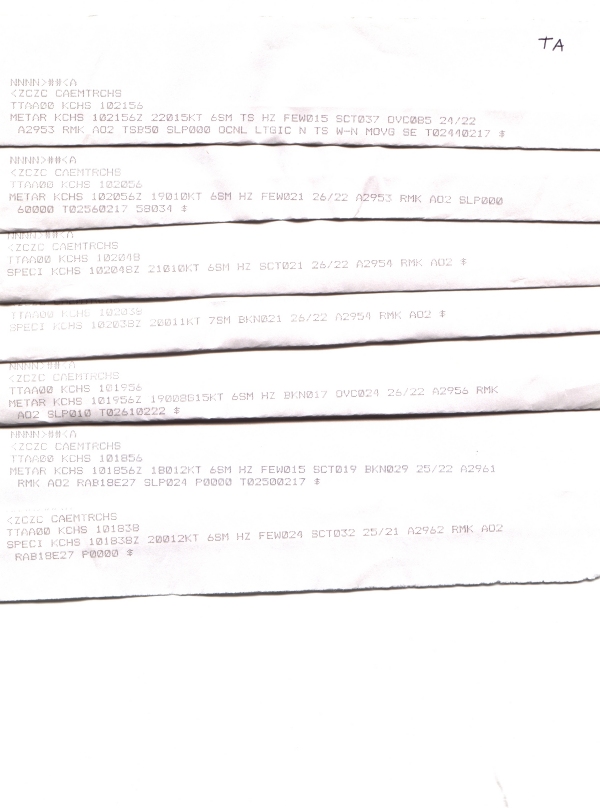
Nevertheless, at 2100, westerly winds were noted from 1000 ft to 3000 ft at increasing speeds from 20 knots to 40 knots. Surface observations at Charleston showed southerly winds with azimuths of 180 deg to 220 deg (FIG TA). The helicity from surface to 1000 ft was obviously impressive with this kind of directional shear. At 2100, surface wind speeds were around 10 knots with gusts to 15 knots while 4000 ft winds were at 35 knots per the Vad Wind Profile. Note that between 2100 and 2138, the 4000 ft winds increased to 45 knots which obviously aided the available speed convergence (FIG VRA). This low level speed max likely reached the area near the time the tornado was at its strongest point west-northwest of the Charleston International Airport.
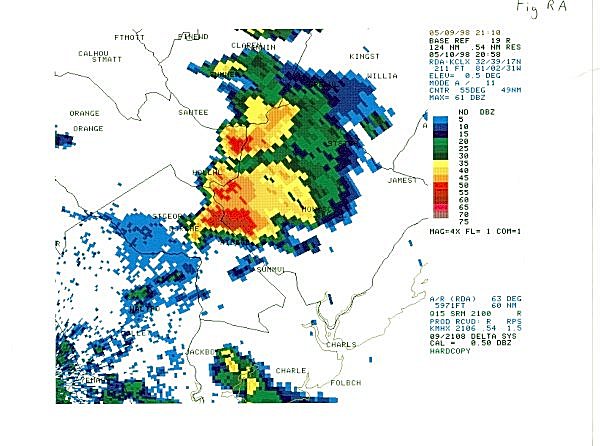
The radar sequence begins at 2058 with a 0.5o base reflectivity product from KCLX approximately 3 minutes after the first wind damage report was received from the town of Rosinville in Dorchester County. Clearly, a classic supercell structure was evident with an intense inflow notch on the southwest flank of the cell giving the appearance of a broad hook echo signature. A rear flank downdraft extended westward from the cell. Note the sharp reflectivity gradient on the inflow side of the storm fueled by a large and vigorous updraft. Unfortunately, an SRM was unavailable at this time, however the wind damage in Rosinville was straight-line and any rotation was likely in the mid levels of the cell (FIG RA).
Shortly after 2100, the soon to be tornadic cell near Ridgeville in Dorchester county produced 0.88 inch diameter hail. The 0.5 deg SRM product from KCLX at 2113 depicted very strong convergence in excess of 50 knots in the low to mid levels of the cell. At this time the cell likely was developing an intense updraft as a forerunner to low level rotation (FIG RB). As the cell continued on an ESE motion, it developed strong mid level rotation as it approached the city of Summerville in southeast Dorchester County.
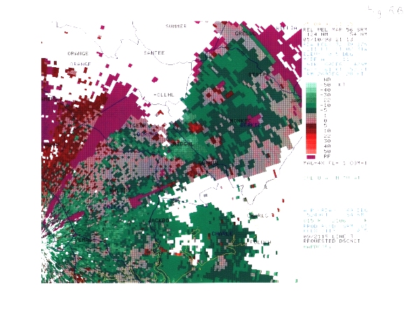
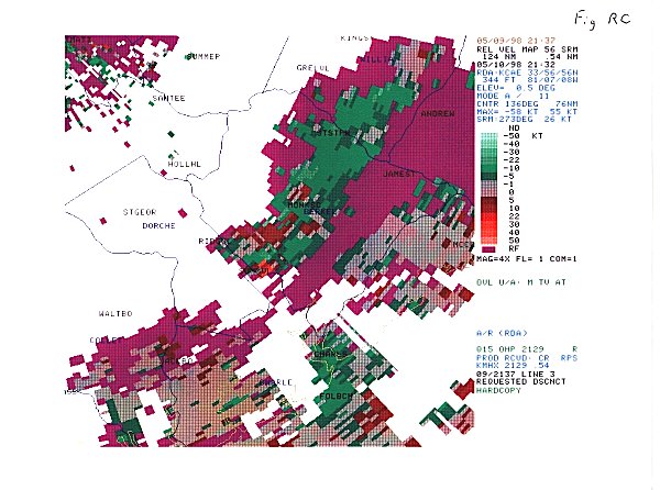
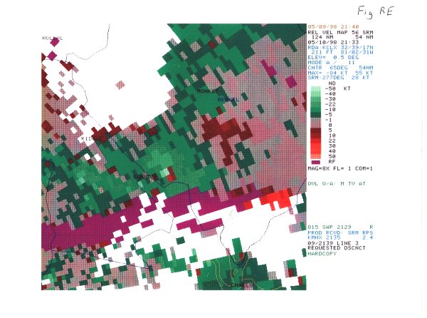
At 2132, the 0.5 deg KCAE SRM depicted strong rotation of near 50 knot over Summerville at approximately the time the tornado was on the ground in the Sangaree subdivision (FIG RC). The 2133 0.5 deg base reflectivity product from KCLX indicated a very complex supercell structure of the tornado producing thunderstorm. Several strong inflow notches were evident on the southwest flank with a distinct rear flank downdraft. Without assistance of the SRM, it may be difficult to pinpoint the updraft/downdraft interface given the complexity of the cell structure. A sharp inflow notch is evident over Summerville with the higher reflectivity associated with the rear flank downdraft located just southeast of Ridgeville (FIG RD). The KCLX 0.5 deg SRM at the same time detected gate to gate rotation just southeast of Summerville having just crossed over into Berkeley County. The distance from the radar was 50 miles while the beam elevation was at 4800 feet. The VR Shear measurement was not available, however given the intensity of the couplet, at least 40 knots of rotation was assumed (FIG RE).
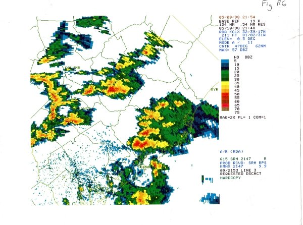
As the thunderstorm progressed east southeast through southern Berkeley County, it continued to rotate, however the 2148 0.5 deg SRM from KCLX showed a more pronounced divergent signature at approximated 5000 feet rather than pure rotation as evidenced in FIG RE. This strong divergent couplet was approximately 8 minutes after wind damage had been observed 15 miles northwest of Jamestown in Berkeley County (FIG RF). In the 0.5 deg reflectivity product at the same time from KCLX, the diminishing reflectivity returns from the rear flank downdraft were still evident east of Summerville and the cell was losing its supercell structure. A weakening rear flanking line was still obvious, however it was most likely phasing into a typical thunderstorm outflow boundary at this time (FIG RG).
As a side note, notice the bowing line of thunderstorms west in FIG RG associated with the tight mid level vorticity maxima approaching from the west of Columbia and Orangeburg. Most of the convection was both near and ahead of the triple point intersection across central South Carolina where the surface low pressure area was deepening.
Seasonal tornado climatology studies for the southeastern United States since 1950 clearly indicate that strong to violent F2 and F3 tornadoes are very unusual in the coastal Carolinas. This event was quite unusual in the fact that both the surface low pressure areas and upper level dynamics moved through South Carolina from west to east, rather that a typical southwest to northeast trajectory. Mid and upper level troughs in the southeast United States usually produce lee side troughs and sharp thermal and moisture boundaries which favor severe weather in the midlands of the Carolinas.
This event was somewhat reminiscent of January or February events across south Georgia and North Florida where warm frontal boundaries are typically located east of ejecting Gulf lows. Missing from this event was strong cold air damming typical seen during the winter months, however favorable low level temperature and moisture gradients played a key role in the development of the Charleston tornado.
NWP guidance strongly suggested a threat of severe weather existed across South Carolina prior to the event but the outlook was clouded by the uncertainty of the amount of de-stabilization to the south of the warm front. As ADAP indicated, very unstable air developed across central and southern coastal South Carolina during the afternoon hours. Enough dynamics were available for the formation of severe thunderstorms producing damaging winds and large hail. An inhibiting factor was the pure west flow aloft as shown on the KCLX Vad Wind Profile.
The wild card was the strength and depth of the surface warm front which was in the vicinity of Charleston. Mesoscale analysis showed extremely tight gradients of moisture and stability in the region where the tornado occurred. The sharp gradient primed the region where low level winds backed and lifted as they entered the warm frontal zone greatly enhancing local helicity as shown in the modified soundings and hodographs.
Finally, radar analysis showed that the thunderstorm that produced the strong tornado underwent several phases during its life cycle. In the mature stage, the cell exhibited classic supercell structure with a large rotating mesocyclone and its inherent severe weather signatures. Other strong cells just north of the main cell may have been a factor in keeping the tornado a short track one, however the interacting effects of adjacent cells is unknown and it would be impossible to model how entrainment affected the complex supercell during its life cycle.
Given the synoptic and mesoscale pattern associated with this event, one gets an impression this event could have been even more serious, possibly producing multiple tornadoes on this day where South Carolina's tornado alley migrated to the coast.
Garinger, L. P., and Knupp, K. R., Seasonal Tornado Climatology for the Southeastern United States, The Tornado: Its Structure, Dynamics, Prediction, and Hazards, p.p. 445-452, Geophysical Monograph Series, 1993.
Przybylinski, R.W., Snow, J.T., Agee, E.M., and Curran, J.T., Seasonal Tornado Climatology for the Southeastern United States, The Tornado: Its Structure, Dynamics, Prediction, and Hazards, p.p. 241-250, Geophysical Monograph Series, 1993.


 Coastal Flood
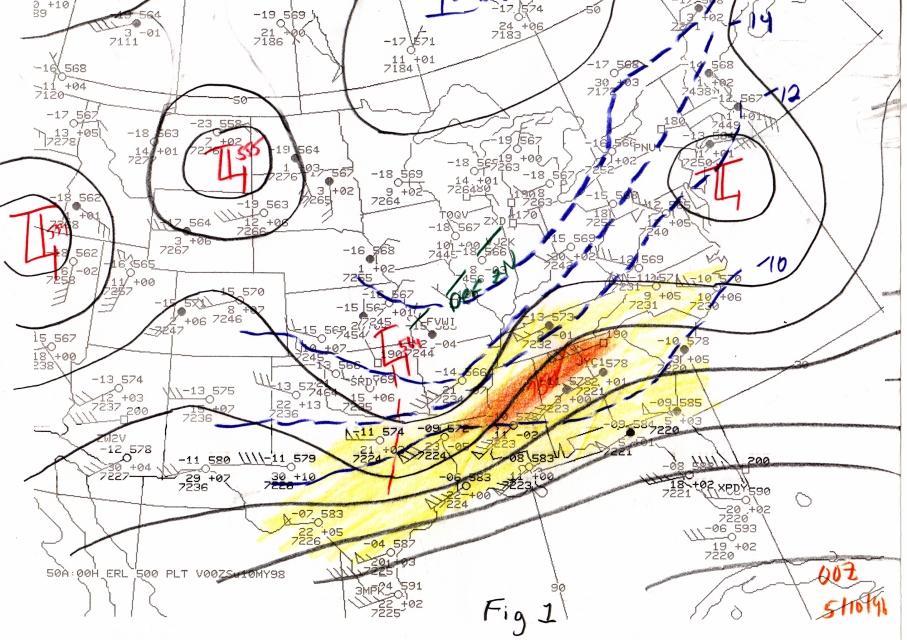