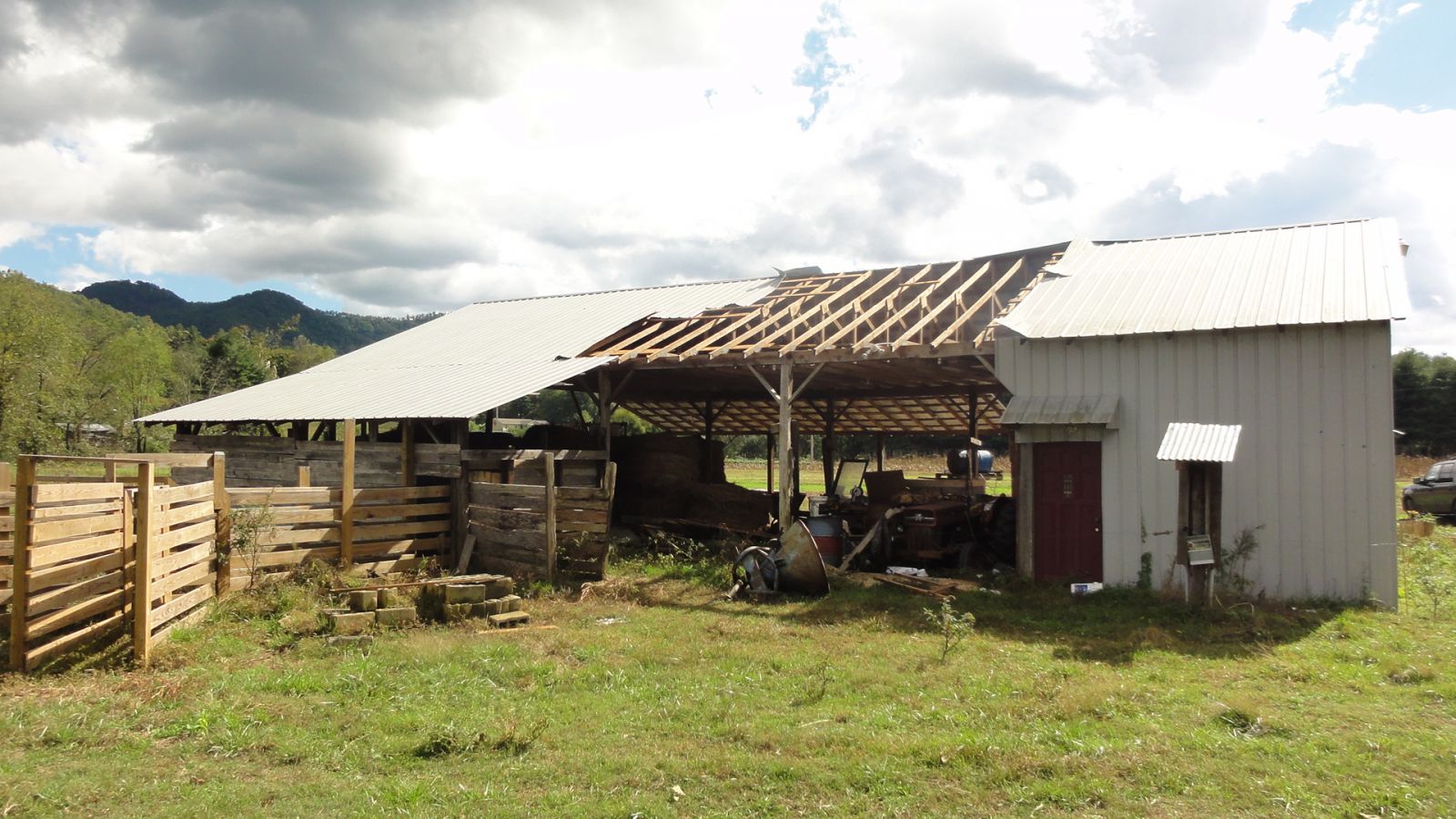
A tornado touched down in McDowell County, North Carolina, in the evening of 14 October 2014, about ten miles south-southwest of Marion along Montford Cove Road.  The tornado was responsible for peeling off part of the metal roof of this outbuilding.

1. Introduction

A severe weather event occurred across the foothills of the Carolinas on 14 October 2014. Three tornadoes touched down on that day, all in relatively close proximity to the Blue Ridge Escarpment (Fig. 1). The first tornado was produced by linear convection during the middle part of the morning over Oconee County, South Carolina, on the grounds of the Fair Play Camp School, located a few miles west of Westminster. The same line of convection also produced wind damage over Stephens County, Georgia, before the tornado and in northern Pickens County, South Carolina, after the tornado. After a long break, a second round of convection crossed Upstate South Carolina during the mid-evening hours. The second tornado touched down near the community of Gowensville, South Carolina, in the northeast corner of Greenville County, at approximately 8 pm Eastern Daylight Time (EDT). The same thunderstorm also produced the third tornado, in McDowell County, North Carolina, about ten miles south-southwest of Marion, at 848 pm EDT (0048 UTC 15 October). The thunderstorm also produced wind damage in between the two tornadoes, near Landrum in extreme northwest Spartanburg County, South Carolina, and after the last tornado, near Morganton in Burke County, North Carolina. The damage from all three tornadoes was rated at EF-0 on the Enhanced Fujita Scale. The tornadoes were produced by thunderstorms that developed in an environment characterized by high amounts of wind shear and low amounts of convective available potential energy (or CAPE, a measure of buoyancy). High shear, low CAPE (HSLC) environments that produce severe weather across the southeastern United States have recently received attention from the academic community (Davis and Parker 2014; Sherburn and Parker 2014; King and Parker 2014).

NOTE: All times from this point forward will be referenced to Universal Time Coordinated (UTC), which is Eastern Daylight Time plus four hours.

Click here to view a list of wind damage, large hail, and tornado reports for this event.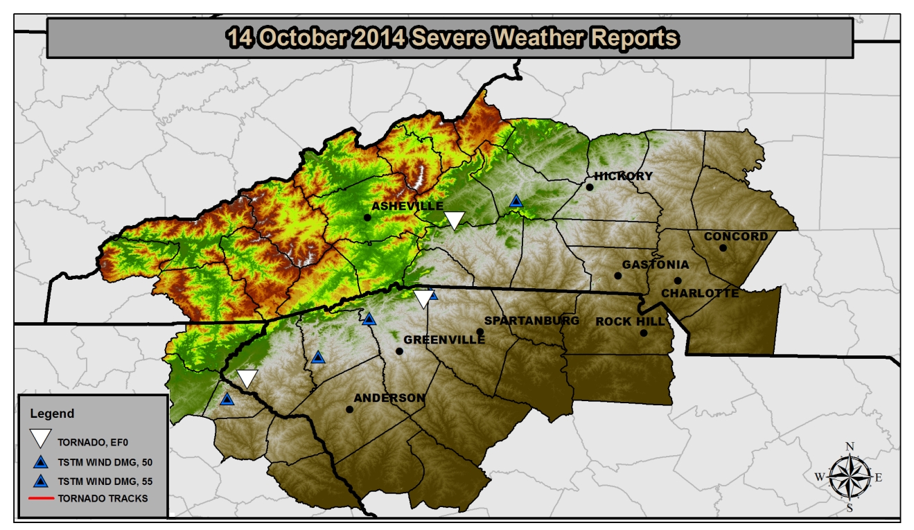

Fig. 1. Tornado, wind damage, and large hail reports for the 24 hour period ending at 1200 UTC on 15 October 2014. Click on image to enlarge.

The potential for severe thunderstorms and tornadoes was well-anticipated by forecasters at the Greenville-Spartanburg (GSP) office of the National Weather Service (NWS) and by forecasters at the Storm Prediction Center (SPC). The forecasters at GSP recognized the signals for a strongly-forced HSLC environment as early as the afternoon of 8 October 2014, as noted in Area Forecast Discussions. The SPC carried a Slight Risk for severe thunderstorms and tornadoes across the GSP county warning area (CWA) beginning with the Day 3 Severe Weather Outlook issued on 12 October. The SPC included a Slight Risk on the subsequent Day 2 Convective Outlooks issued on 13 October. That the occurrence of three tornadoes met with the expectations of the forecast of severe weather in an HSLC environment was perhaps the most interesting aspect of this case. Another facet was the relatively long duration of the severe thunderstorm threat. Most of the GSP CWA was under a Tornado Watch that began in the early morning and then continued through the late afternoon and evening hours. The two episodes of severe weather were separated by nearly 12 hours, which allowed the convective environment to destabilize in the interim.

2. Synoptic Features

The environment across the western Carolinas and northeast Georgia was expected to be favorable for severe thunderstorms and tornadoes, as noted in the Day 1 Convective Outlook issued by the SPC in the early morning hours on 14 October. The upper air pattern on 14 October 2014 featured a high-amplitude trough over the Mississippi River basin and a ridge off the east coast of North America. The upper trough-ridge system provided for deep southerly flow of moisture from the Gulf of Mexico ahead of a strong cold front. The right entrance region of a meridional upper jet streak, exceeding 110 kt at the 300 hPa level (Fig. 2), brought upper divergence across the western Carolinas at 1200 UTC on 14 October, which continued throughout the day. At 500 hPa, a series of short waves swinging around the base of the upper trough and across the Mississippi Delta region at 1200 UTC (Fig. 3) changed the tilt of the upper trough axis from positive to negative during the day, effectively increasing upper difluence downstream over the western Carolinas by 0000 UTC on 15 October (Fig. 4). A mid-level jet streak in the 70-90 kt range also contributed to an increase in vertical wind shear in the afternoon and evening. The 700 hPa analysis showed a tight west-to-east gradient of moisture coincident with the core of strongest winds (about 50 kt) moving eastward across Georgia and the western Carolinas at 0000 UTC on 15 October (Fig. 5). Water vapor satellite imagery detected the short waves at 2045 UTC as a train of westward-bulging waves in the mid-level moisture gradient stretching from Michigan to the Florida Panhandle (Fig. 6). Other studies of HSLC events have noted a strengthening of convection as a mid-level dry air intrusion moves over a highly sheared but weakly buoyant low level environment (Lane and Moore 2006; Clark 2009; Evans 2010), thought to be related to a release of potential instability. The tight gradient of moisture also appeared on the 850 hPa analysis at 0000 UTC on 15 October (Fig. 7), along with a backing 40 kt low level jet which increased the low level wind shear ahead of the convective line. The nearly vertically stacked upper low centered over Illinois during the afternoon of 14 October slowed the forward progress of the trough, which contributed to the long duration of the severe thunderstorm threat.

Click here to view an 30 frame Java loop of GOES-13 Water Vapor satellite images from 0545 UTC on 14 October to 1145 UTC on 15 October 2014.

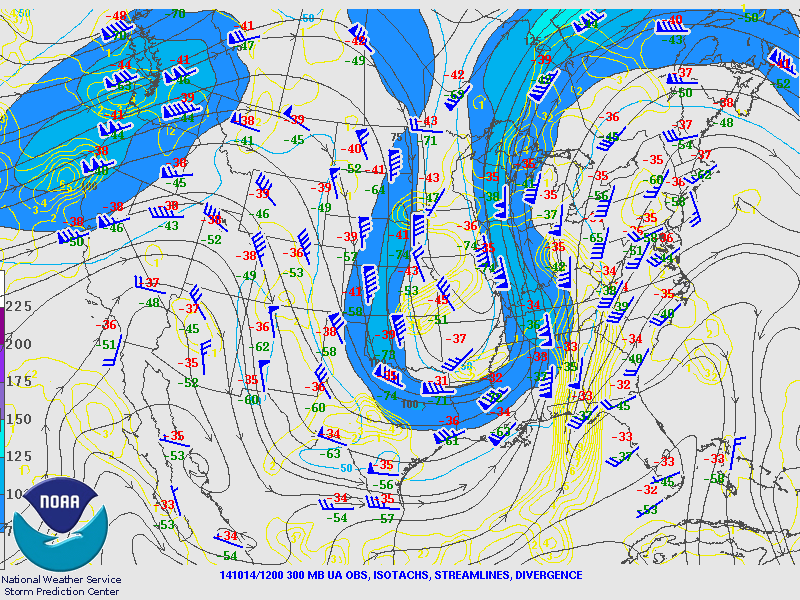
Fig. 2. SPC objective analysis of 300 hPa isotachs (kt; blue contours, color fill greater than 70 kt), wind (kt; barbs), streamlines (gray contours with arrow showing direction of motion), and divergence (s⁻¹ ; yellow contours) at 1200 UTC on 14 October. Click on image to enlarge.

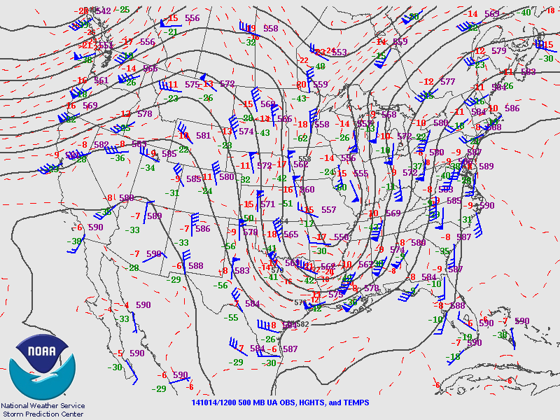
Fig. 3. SPC objective analysis of 500 mb geopotential height (dm; dark gray contours), temperature (°C; dashed red contours), and wind (kt; barbs) at 1200 UTC on 14 October 2014. Click on image to enlarge.

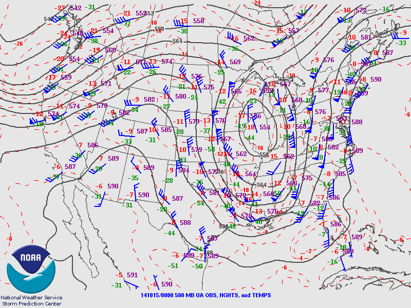
Fig. 4. As in Fig. 3, except for 0000 UTC on 15 October 2014. Click on image to enlarge.

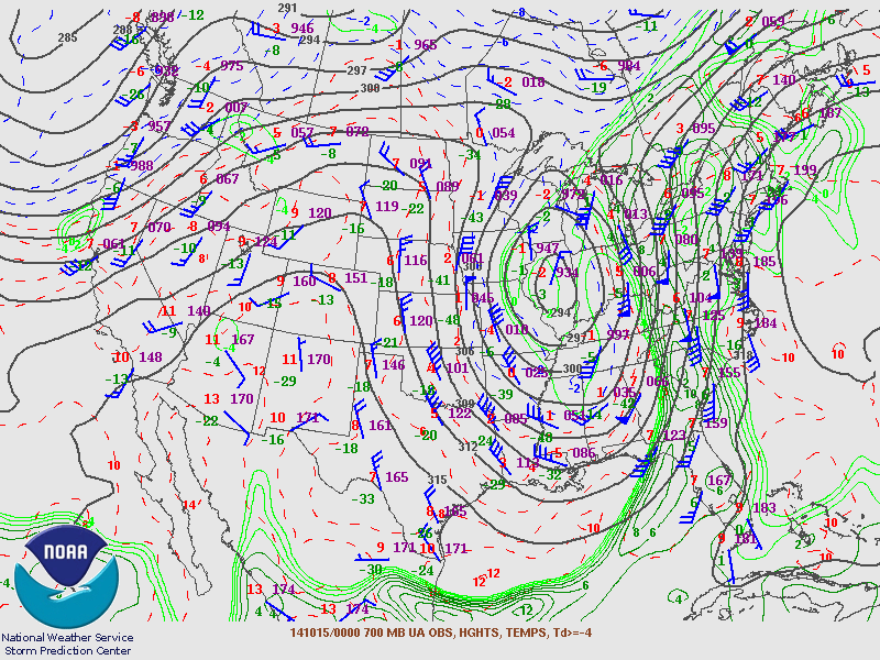
Fig. 5. SPC objective analysis of 700 hPa geopotential height (dm; gray contours), temperature (°C; dashed red contours), wind (kt; barbs), and dewpoint (°C; green contours above -4) at 0000 UTC on 15 October 2014. Click on image to enlarge.

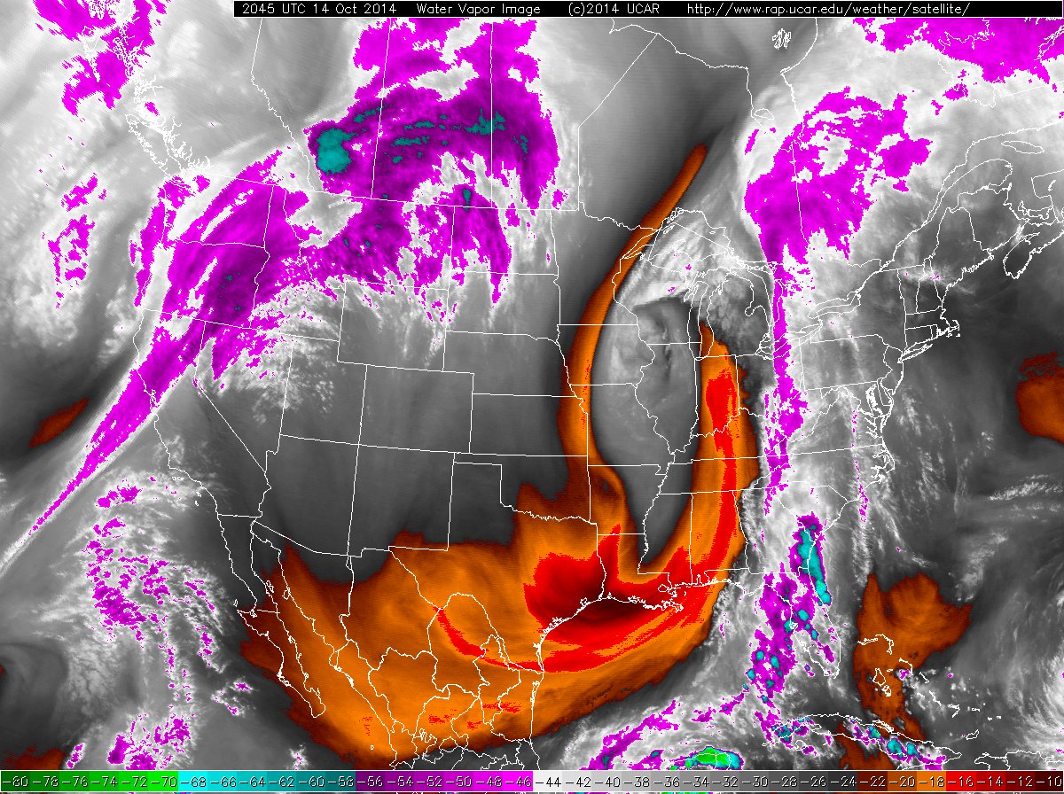
Fig. 6. GOES composite water vapor satellite imagery at 2045 UTC on 14 October 2014. Brightness temperatures are shown by the color table at the bottom. Click on image to enlarge.

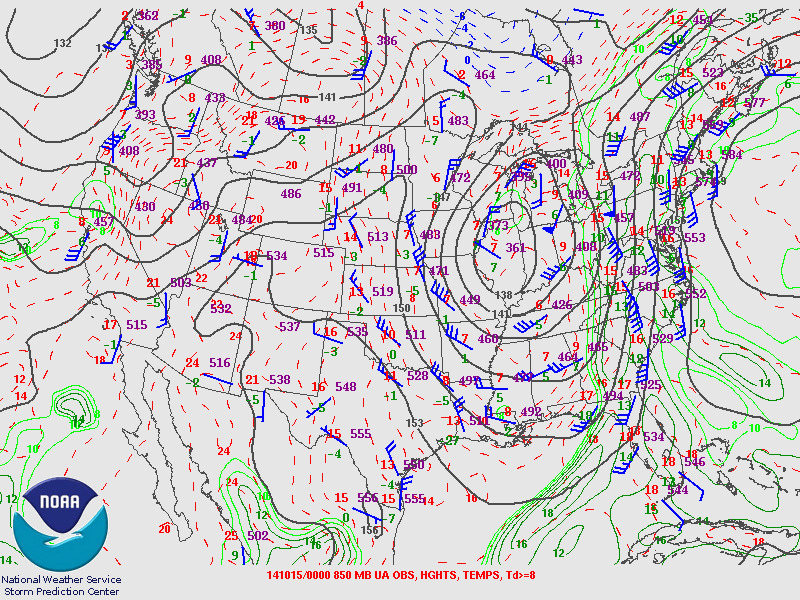
Fig. 7. SPC objective analysis of 850 hPa geopotential height (m; gray contours), temperature (°C; dashed red contours), wind (kt; barbs), and dewpoint (°C; green contours above 8) at 0000 UTC on 15 October 2014. Click on image to enlarge.

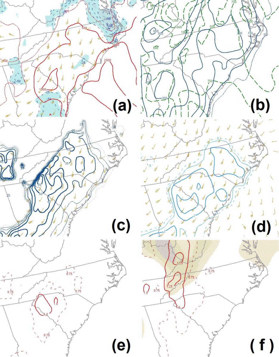
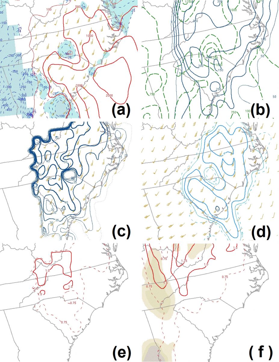
The verification of the forecast on 14 October 2014, in which a tornado-producing quasi-linear convective system (QLCS) formed in an HSLC environment as expected, provided an interesting comparison with recent events that failed to meet the expectations of forecasters at NWS GSP. On at least three occasions in the past three years, forecasters at GSP expected severe weather to occur in an HSLC environment, yet little or no damage was reported (Fig. 8). On 10 December 2012, the passage of a southwest-to-northeast oriented cold front produced a wide, broken band of showers with embedded thunderstorms that did not produce severe weather in the GSP CWA, although some wind damage occurred in Alabama. On 22 December 2013, a wide band of showers and thunderstorms moved slowly east across the GSP CWA. One report of wind damage was received over Gaston County, North Carolina, but that was the only report of severe weather across the United States that day. On 14 April 2014, a decaying mesoscale convective system (MCS) crossed the GSP CWA in the afternoon without producing severe weather, although isolated wind damage was reported in eastern North Carolina. During the early morning hours on the following day, a broken band of showers and non-severe thunderstorms moved across the area ahead of a cold front. In each case, the 500 mb height pattern, analyzed from the most recent upper air data collected prior to the time convection moved across the GSP CWA, featured a trough axis along or west of the Mississippi river and southwesterly flow aloft with a jet core northwest of the southern Appalachians (Fig. 9). However, on 14 October 2014, the axis of a relatively higher amplitude trough was located east of the Mississippi River along with a more southerly mid-level jet core over the southern Appalachians. The water vapor imagery, taken at the time convection reached the GSP CWA, showed evidence of a southwesterly flow at mid-levels of the atmosphere and a moisture gradient that was weak or located several hundred kilometers west of the GSP CWA in the three "non-event" cases (Fig. 10). However, the water vapor imagery on 14 October 2014 showed a much stronger, more west-to-east oriented gradient in closer proximity to the severe weather. In all three "non-event" cases, at the 3-hourly synoptic time prior to the passage of convection, a surface cold front was analyzed several hundred kilometers west of the GSP CWA in a southwest to northeast orientation. On 14 October 2014, the cold front was in closer proximity to the location of severe weather and featured a more meridional orientation (Fig. 11). The comparisons of surface front orientation, mid-level moisture gradient, and 500 mb trough orientation suggest that the magnitude and organization of synoptic scale forcing may play a role in discriminating between HSLC environments that produce severe weather and environments that do not.

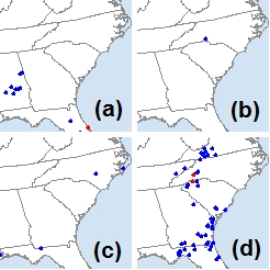
Fig. 8. Preliminary local storm reports received for the 24 hour period beginning at 1200 UTC on (a) 10 December 2012, (b) 22 December 2013, (c) 14 April 2014, and (d) 14 October 2014. Blue dots indicate wind damage and red dots indicate tornado locations.

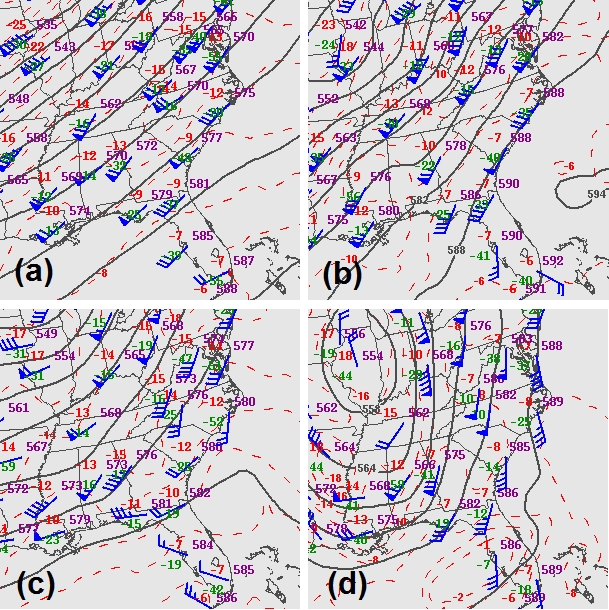
Fig. 9. SPC Objective analysis of 500 mb geopotential height (dm; gray contours), temperature (°C; dashed red contours), and wind (kt; barbs) at (a) 1200 UTC on 10 December 2012, (b) 1200 UTC on 22 December 2013, (c) 1200 UTC on 14 April 2014, and (d) 0000 UTC 15 October 2014. Click image to enlarge.

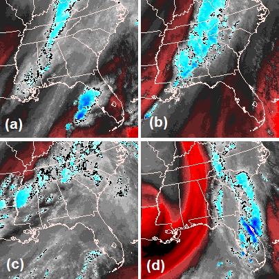
Fig. 10. GOES-13 water vapor channel imagery at (a) 1745 UTC on 10 December 2012, (b) 1745 UTC on 22 December 2013, (c) 1745 UTC on 14 April 2014, and (d) 2345 UTC on 14 October 2014. Click image to enlarge.

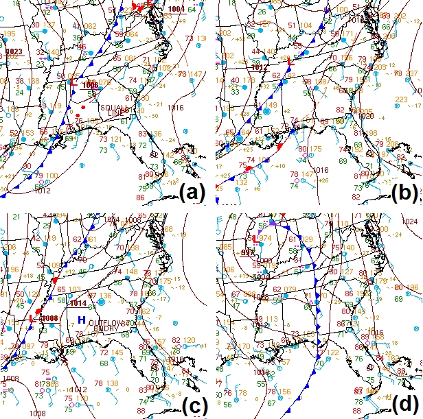
Fig. 11. Hydrometeorological Prediction Center analysis of mean sea level pressure (mb; black contours) and surface fronts (standard symbols) at 1800 UTC on (a) 10 December 2012, (b) 22 December 2013, (c) 14 April 2014, and (d) 14 October 2014. Click image to enlarge.

The first round of thunderstorms on 14 October 2014 moved across Georgia as an MCS in the pre-dawn hours well ahead of the surface cold front. The leading edge of the MCS was shown by radar just west of the Savannah River at 1200 UTC on 14 October (Fig. 12). An upper air sounding taken at Peachtree City, Georgia, at 1200 UTC on 14 October was contaminated by the trailing stratiform region of the MCS (Fig. 13). However, the sounding still showed nearly 200 J kg⁻¹ of CAPE for the most unstable parcel (MUCAPE), along with strong shear (54 kt) in the surface to 3 km AGL layer. The SPC mesoanalysis at 1200 UTC (Fig. 14) showed the environment along and ahead of the MCS across western South Carolina was characterized by MUCAPE closer to 500 J kg⁻¹ and effective shear in the 45-55 kt range. Both values were in the range of what Davis and Parker (2014) and Sherburn and Parker (2014) consider being an HSLC environment. The storm relative helicity (SRH) was in the 200-300 m²s⁻² range and the lifting condensation level (LCL) was relatively low (around 500 m). The supercell composite parameter was greater than 1, suggesting the environment was favorable for right-moving supercells. An experimental parameter to diagnose severe weather in HSLC environments, known as SHERB (Severe Hazards in Environments with Reduced Buoyancy), indicated values greater than 1 across western South Carolina, which suggested the potential for an increased risk of damaging wind gusts and tornadoes (Sherburn and Parker, 2014). Based on the favorable environment ahead of the MCS, the SPC kept most of the region in the Slight Risk on the updated Day 1 Convective Outlook valid at 1300 UTC.

Fig. 12. Mosaic of radar composite reflectivity (dBZ; color fill, table at bottom) at 1200 UTC on 14 October 2014. Source: UCAR/NCAR. Click to enlarge.

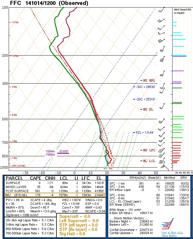
Fig. 13. Skew-T, log P diagram for upper air sounding taken at Peachtree City, Georgia (FFC), at 1200 UTC on 14 October 2014. The temperature sounding is shown by the thick red line and the dewpoint sounding is shown by the thick green line. A table of convective parameters is shown at the bottom. Click to enlarge.

Fig. 14. SPC mesoanalysis of (a) most unstable CAPE (J kg⁻¹ ; red contours), most unstable convective inhibition (J kg⁻¹ ; dashed blue contours and color fill), and effective bulk shear (kt; barbs), (b) 0-1 km SRH (m²s⁻²; blue contours) and 100 mb mean LCL (m; green contours), (c) effective bulk shear (kt, blue contours and barbs), (d) effective layer supercell composite parameter (light blue contours) and storm motion (kt; barbs), (e) SHERBe (red contours), and (f) 0-3km SHERB (red countours) and lifted index (color fill) at 1200 UTC on 14 October 2014. Click to enlarge.

The initial wave of convection weakened during the middle to late part of the morning as it moved east across upstate South Carolina, although the environment was still expected to be favorable for severe thunderstorms and a few tornadoes later in the day. New thunderstorms developed over western Georgia in the early afternoon closer to the cold front where forcing was strongest. The new development spurred the SPC to issue a new Tornado Watch for the western Carolinas for the rest of the afternoon and evening, as the environment remained favorable ahead of the cold front.

A surface cold front moving slowly east across the western North Carolina and north Georgia provided the focus for the development of a second line of convection in a favorable environment for severe thunderstorms and tornadoes over Upstate South Carolina and northeast Georgia during the evening hours (Fig. 15).  An upper air sounding taken at Greensboro, North Carolina (GSO), at 0000 UTC on 15 October (Fig. 16) sampled the pre-frontal air mass well. Surface-based CAPE and MUCAPE exceeded 800 J kg⁻¹, more than sufficient to support a tornadic QLCS. SRH was greater than 250 m²s⁻² in the layer from the surface to 3 km AGL, which suggested an increased tornado threat. Bulk shear in the same layer was 37 kt, which also indicated an increasing risk of supercells and severe thunderstorms. The SPC mesoanalysis at 2300 UTC (Fig. 17) showed the environment ahead of the second line was not much different than the environment earlier in the day. The MUCAPE across Upstate South Carolina was still less than 500 J kg⁻¹ and effective bulk shear was close to 45 kt. A sounding from the initialization of the 15 October 2014/0000 UTC run of the Rapid Refresh (RAP) model, taken from a point near Hickory, North Carolina (HKY), revealed a more typical cool season HSLC convective environment (Fig. 18). The sounding showed a low LCL of 522 m, 100 hPa mixed layer CAPE (MLCAPE) of 152 J kg⁻¹, 0-3 km shear of 47 kts, and 0-1 km SRH of 379 m²s⁻². Thus, in spite of what the GSO sounding indicated, the pre-storm environment remained within the HSLC thresholds outlined by Davis and Parker (2014). The SHERB parameter was between 0.75 and 1.0, which was less than the earlier values, but still within the range of values associated with an increased likelihood of severe weather reports in an HSLC environment.

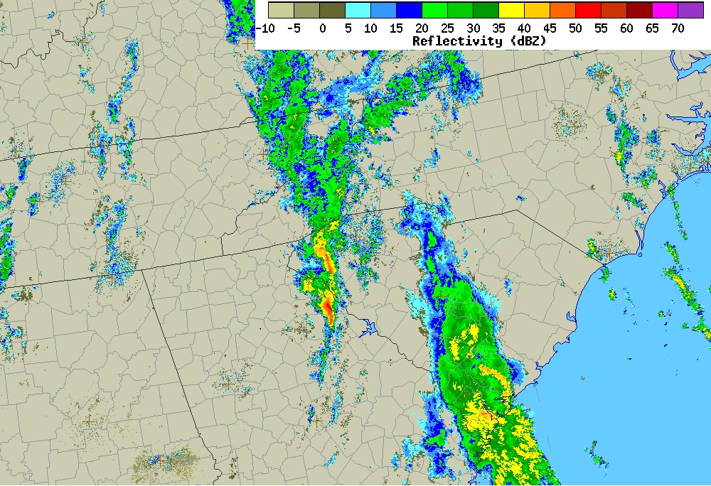
Fig. 15. As in Fig. 12, except for 2300 UTC on 14 October 2014. Click to enlarge.

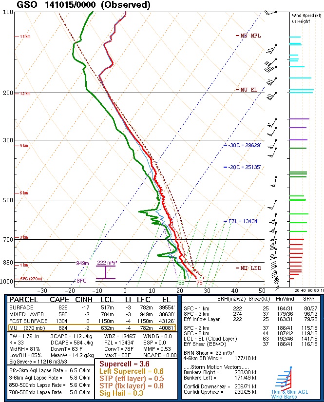
Fig. 16. As in Fig. 13, except for Greensboro, North Carolina (GSO), at 0000 UTC on 15 October 2014. Click to enlarge.

Fig. 17. As in Fig. 14, except at 2300 UTC on 14 October 2014. Click to enlarge.

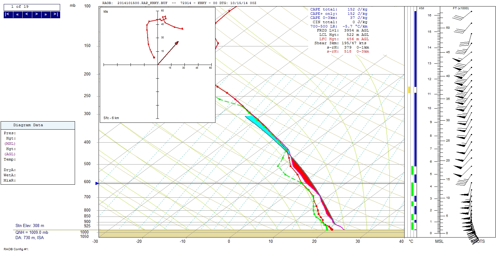
Fig. 18. Skew-T/log-p plot of a sounding near the Hickory Regional Airport (KHKY) from the 15 October 2014 initilization of the RAP model. The hodograph and CAPE analysis are presented as well. The CAPE caclulation uses the virtual temperature correction method. The area shaded in red is the positively buoyant area of the sounding. The light blue shade represents negative buoyancy. Click to enlarge.

Click here to view an 13 frame Java loop of HPC surface maps from 0000 UTC on 14 October to 1200 UTC on 15 October 2014.

3. Radar Overview

a.  The Fair Play Camp School Tornado

A relatively small QLCS moved across northeast Georgia during the early morning hours on 14 October 2014. By 1151 UTC, a ragged-looking band of high reflectivity (greater than 45 dBZ) extended southward from Toccoa, Georgia, and was about to move into South Carolina (Fig. 19). The two lowest scans showed evidence of a rear-inflow notch manifested as the concave appearance on the west flank of the system. The normalized rotation (NROT) product from GR2Analyst peaked at 0.85 on the 0.5 degree scan (Fig. 20), while increasing storm relative velocity (SRV) prompted the issuance of a Tornado Warning for portions of Stephens County, Georgia, and Oconee County, South Carolina.

Click here to view an 10 frame Java loop of a regional mosaic of radar reflectivity from 0600 UTC to 1500 UTC on 14 October 2014.

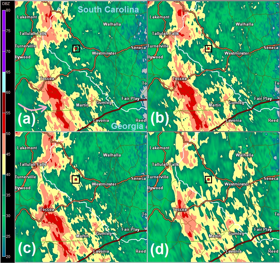
Fig. 19. KGSP base reflectivity on the (a) 0.5 degree, (b) 0.9 degree, (c) 1.3 degree, and (d) 1.8 degree scan at 1151 UTC on 14 October 2014. The red square inside the black box indicates the location of the Fair Play Camp School, west of Westminster, South Carolina. The pink arrow indicates the location of a weak echo channel. The white contour denotes the border between South Carolina and Georgia. Reflectivity values (dBZ) are indicated by the color bar on the left side of the figure. Click to enlarge.

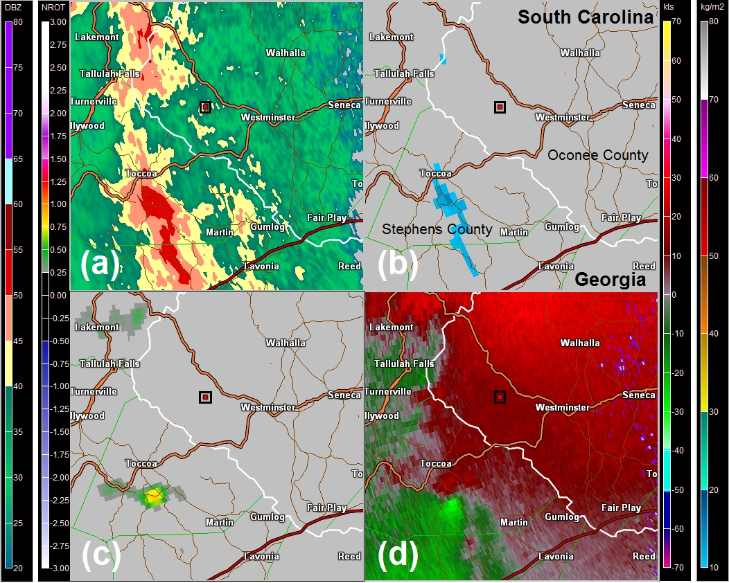
Fig. 20. KGSP 0.5 degree scan of (a) base reflectivity (dBZ), (b) digital vertically integrated liquid (VIL), (c) NROT, and (d) SRV (kt) at 1151 UTC on 14 October 2014. Values of reflectivity and NROT are shown by the color tables on the left side of the figure and values of SRV and VIL are shown by the color tables on the right side of the figure. County borders are shown as thin light green lines. The location of the Fair Play Camp School is shown by the red square inside the black box. Click to enlarge.

The reflectivity pattern acquired a more "S-shaped" pattern by 1201 UTC as the QLCS crossed the state border (Fig. 21). A weak echo channel developed on the lowest three elevation scans and was wrapping around the southern flank of the trailing segment of the QLCS, while the leading line segment bowed northeastward across the area to the west of Westminster, South Carolina. Values of NROT decreased to 0.73 on the lowest scan (Fig. 22). Rotation was insignificant on the 1.3 degree scan and above.

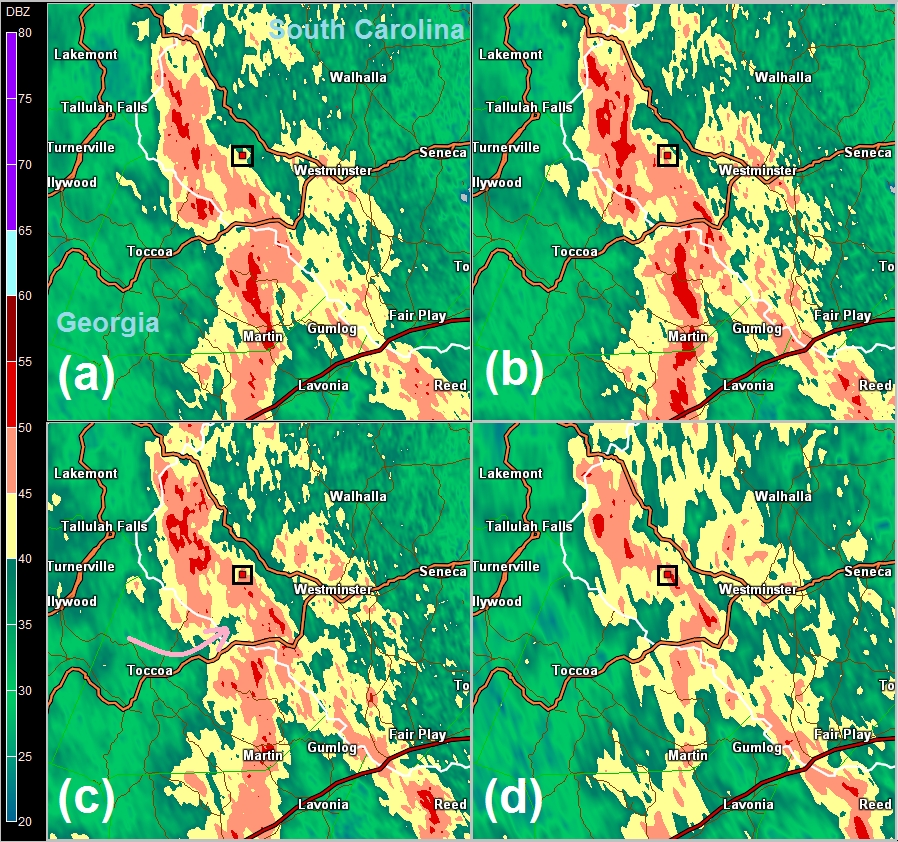
Fig. 21. As in Fig. 19, except for 1201 UTC. The pink arrow in (c) shows the location of the weak echo channel. Click to enlarge.

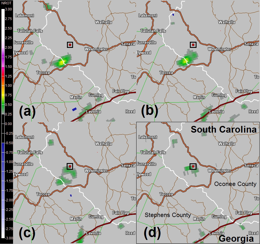
Fig. 22. NROT from the KGSP radar on the (a) 0.5 degree, (b) 0.9 degree, (c) 1.3 degree, and (d) 1.8 degree scan at 1201 UTC on 14 October 2014. The values of NROT are given by the color table on the left side of the figure. Click to enlarge.

The Supplemental Adaptive Intra-Volume Low-Level Scan (SAILS) data at 1209 UTC, about two minutes before tornadogenesis, showed a more prominent forward surge of the bowing reflectivity segment of the QLCS, with a weak echo channel surging ahead of the trailing reflectivity segment (Fig 23). Although NROT remained steady at 0.73, low level rotation remained broad. The tornado touched down on the grounds of the Fair Play Camp School, about three miles west of Westminster, at 1211 UTC. The KGSP radar showed the strongest rotation coincident with the southern tip of the trailing reflectivity segment and a weak echo channel wrapped around the southern end.

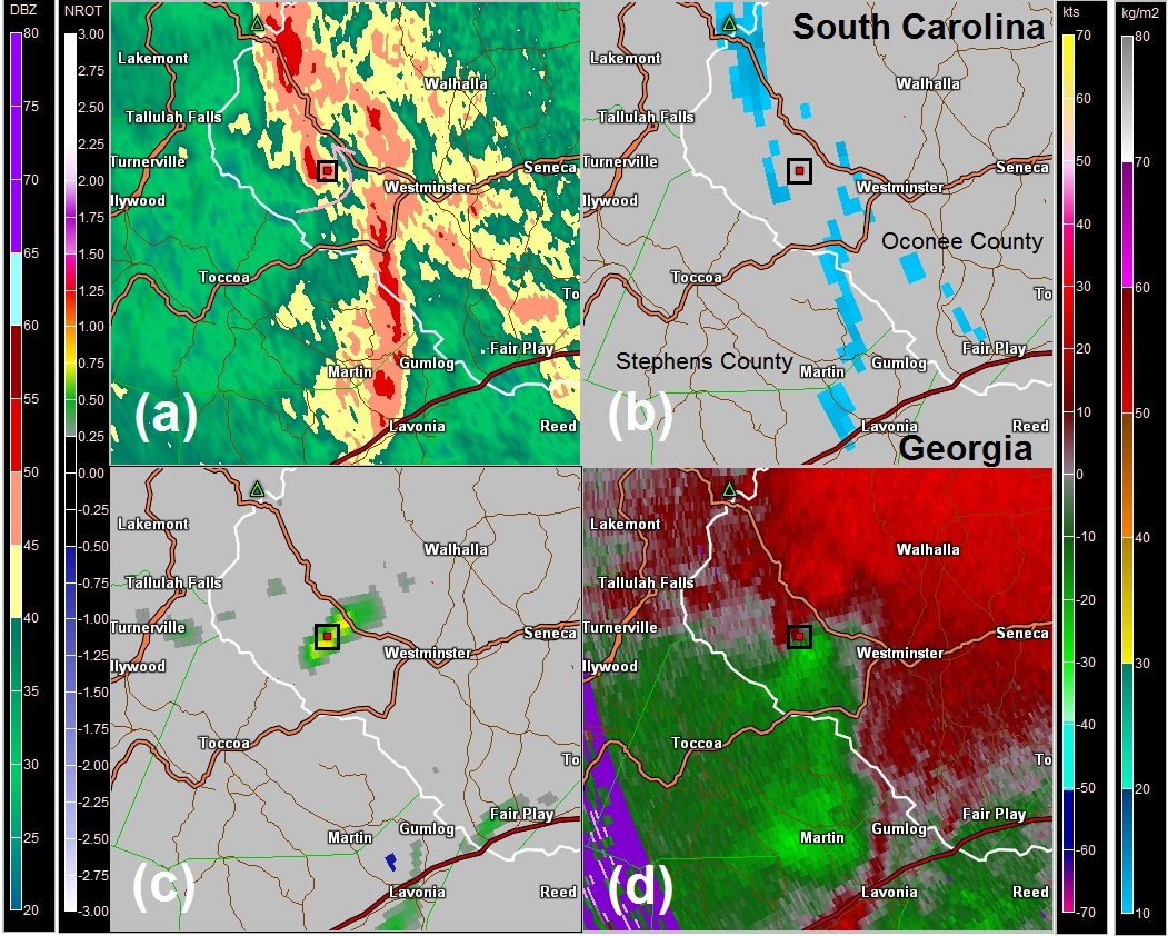
Fig. 23. As in Fig. 20, except for 1209 UTC. Click to enlarge.

b.  The Gowensville Tornado

At 2348 UTC on 14 October, a second QLCS was moving across Upstate South Carolina, specifically Greenville County (Fig. 24). Reflectivity imagery did not reveal any significant features, although the QLCS was well organized with a strong reflectivity gradient along the forward flank. SRV images revealed an elongated axis of vertical cyclonic shear associated with the gust front (Fig. 25). While SRV revealed no organized areas of significant cyclonic rotation in the lowest levels, the velocity structure became more rotational with height, especially above 1500 m (about 5000 ft) AGL. The NROT product (Fig. 26) from GR2Analyst quantified this shear as being quite robust, with some values exceeding 1.0, especially above 0.5 degrees. However, at this time the NROT was strung out along the shear axis, typical of strong gust fronts.

Click here to view an 16 frame Java loop of a regional mosaic of radar reflectivity from 1500 UTC on 14 October 2014 to 0600 UTC on 15 October 2014.

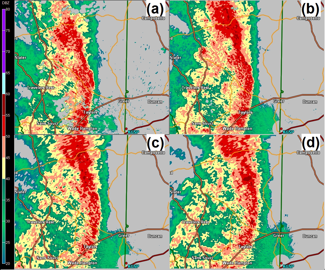
Fig. 24. KGSP base reflectivity imagery at (a) 0.5 degrees, (b) 1.3 degrees, (c) 2.4 degrees and (d) 4.0 degrees at 2348 UTC on 14 October. The vertical green line indicates the boundary between Greenville County (west) and Spartanburg County (east), South Carolina. The location of the KGSP radar is shown by the red dot in the lower right corner of each panel. Click to enlarge.

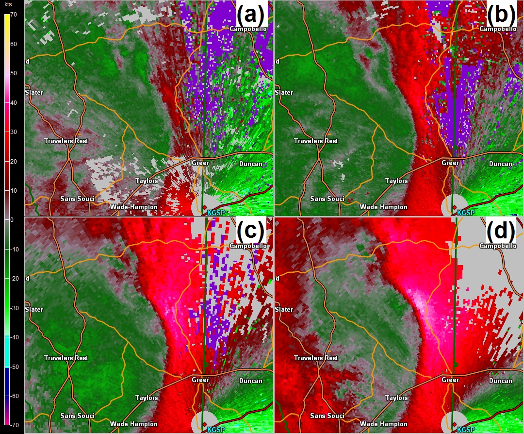
Fig. 25. As in Fig. 24, except for SRV. Values of SRV are given by the color table on the left side of the figure. Click to enlarge.

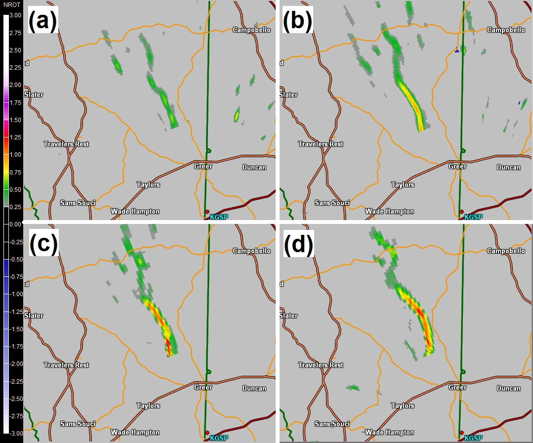
Fig. 26. As in Fig. 24, except for NROT. The values of NROT are given by the color table on the left side of the figure. Click to enlarge.

At 2354 UTC, reflectivity imagery from KGSP (Fig. 27) showed a slight bowing structure over northern Greenville County, with a notch in the forward flank of the QLCS just north of the bow. A small area of weak rotation was observed on the NROT product at 0.5 degrees where the notch intersected the reflectivity field (Fig. 28). This rotation tilted toward the northeast and increased significantly with height, with NROT maximized at 0.93 at 2.4 degrees (1.0 km AGL). The circulation was not observed above 1.8 km AGL. One interesting aspect of the NROT products was the fracture in the elongated shear axis on the lowest two elevation scans between 2348 UTC and 2354 UTC, which occurred approximately six minutes prior to tornadogenesis.

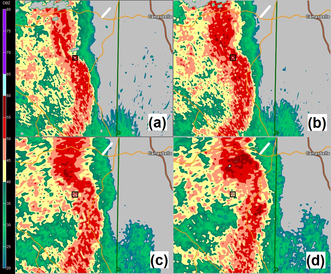
Fig. 27. KGSP base reflectivity imagery at (a) 0.5 degrees, (b) 0.9 degrees, (c) 1.8 degrees, and (d) 3.1 degrees at 2354 UTC on 14 October 2014. The white line represents the path of the Gowensville tornado. The pink square inside the black box is centered over the maximum NROT at 0.5 degrees. Click to enlarge.

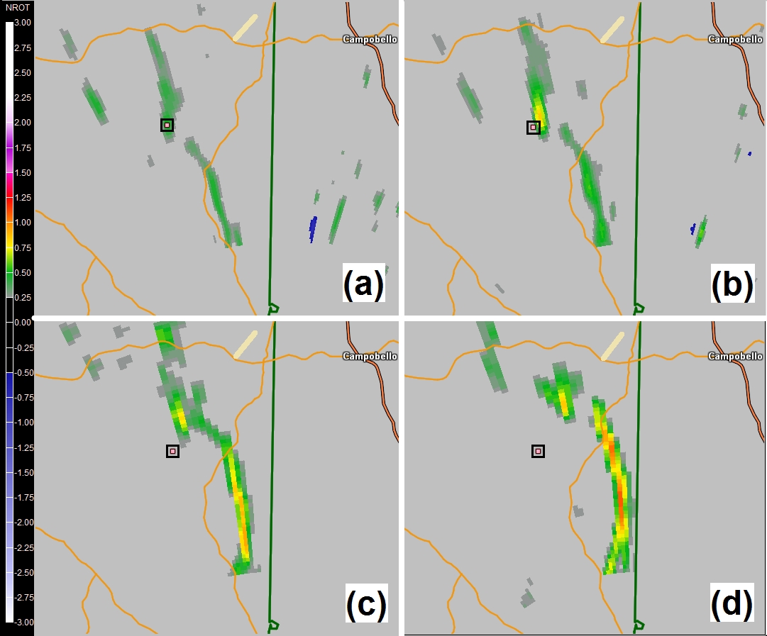
Fig. 28. NROT product from GR2Analyst from KGSP radar scans at (a) 0.5 degrees, (b) 0.9 degrees, (c) 1.8 degrees, and (d) 3.1 degrees at 2354 UTC on 14 October 2014. The pink square inside the black box indicates the maximum in NROT on the 0.5 degree scan. The light yellow line indicates the track of the Gowensville tornado. Click to enlarge.

By 2357 UTC, the SAILS scan (Fig. 29) indicated the bow/notch pair had become more prominent, while the circulation had strengthened substantially at 0.5 degrees (~200 m AGL). In fact, the strongest rotation associated with this mesovortex (0.97) was now observed at this level. The forward flank notch filled with reflectivity at the lowest elevation scans by 2359 UTC (Fig. 30). At higher elevations scans (e.g., 3.1 degrees), a "bulb" of high reflectivity was observed in the vicinity of the remnant mesovortex. North of this feature, the high reflectivity region was becoming more disorganized and fragmented. About a minute before the tornado (2359 UTC, Fig. 31), the mesovortex had weakened considerably above 400 m AGL, while rotation remained significant at 0.5 degrees, where NROT was 0.97.

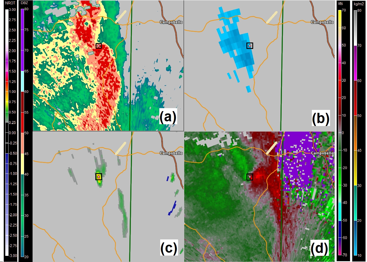
Fig. 29. KGSP scans of (a) 0.5 degree base reflectivity, (b) digital VIL, (c) NROT, and (d) SRV from the SAILS scan at 2357 UTC on 14 October, except for digital VIL which is from the 2354 UTC scan. The pink square inside the black box denotes the location of the highest NROT on the 0.5 degree scan. Click to enlarge.

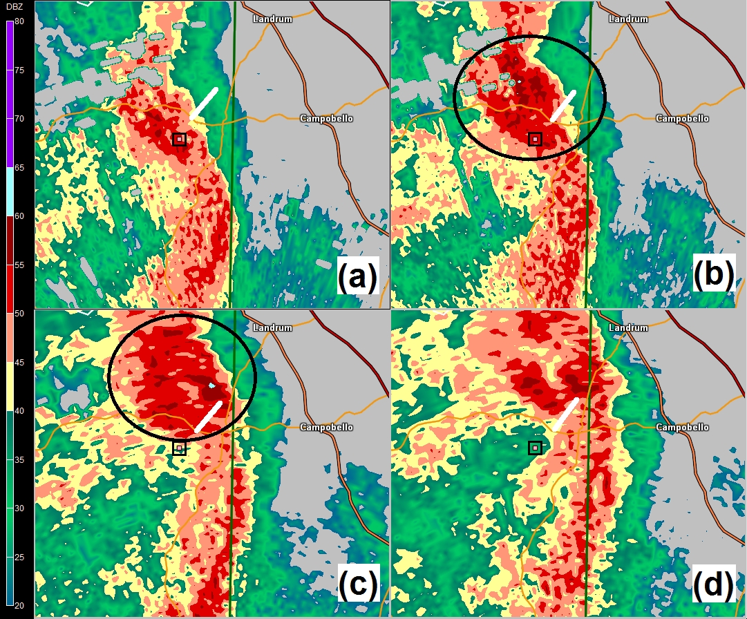
Fig. 30. As in Fig. 27, except for 2359 UTC. The pink square inside the black box indicates the maximum NROT on the 0.5 degree scan. The black oval highlights the reflectivity bulb. The track of the Gowensville tornado is indicated by the white line. Click to enlarge.

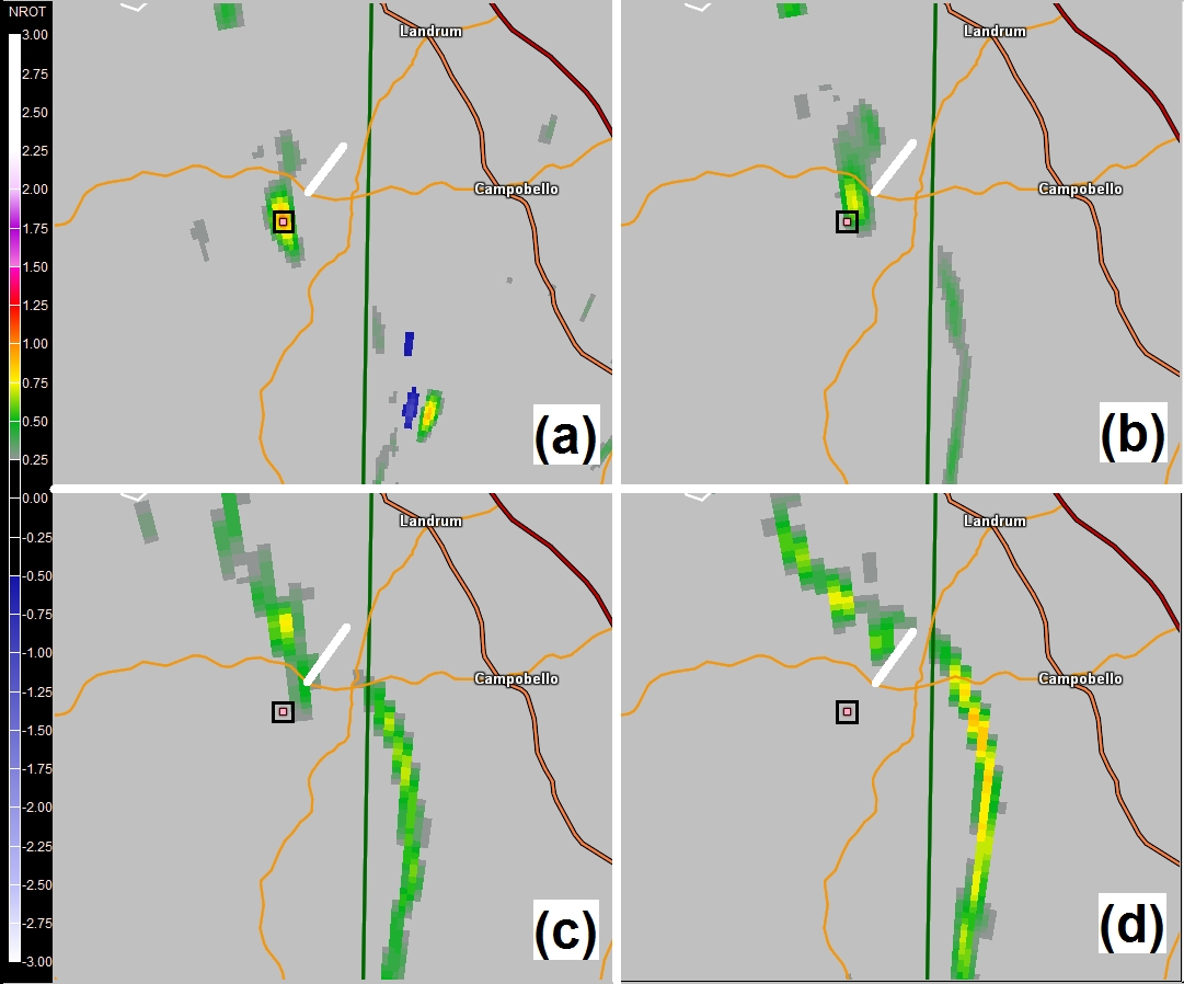
Fig. 31. As in Fig. 28, except at 2359 UTC. The pink square inside the black box denotes the maximum NROT on the 0.5 degree scan in (a). Click to enlarge.

The QLCS continued to weaken through 0010 UTC on 15 October. A reflectivity bulb was observed on the 0.5 degree scan (Fig. 32), very similar to that seen aloft at 2359 UTC. Meanwhile, the QLCS completely fractured into two high reflectivity segments aloft (Fig. 33), but ten minutes after the Gowensville tornado touched down and more than 15 minutes after the fracture was noted in the NROT field. The digital vertically integrated liquid (VILD) product between 2354 UTC on 14 October and 0015 UTC on 15 October illustrated the weakening evolution quite well (Fig. 34).

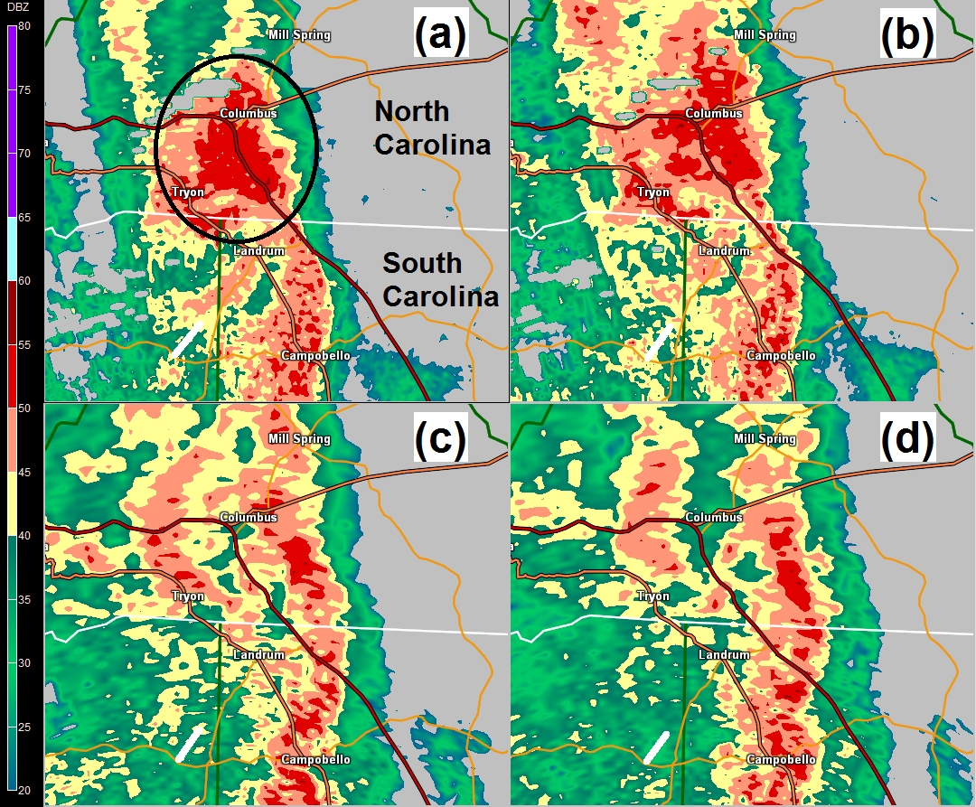
Fig. 32. As in Fig. 27, except at 0010 UTC on 15 October 2014. The black oval highlights the reflectivity bulb on the 0.5 degree scan in (a). The white contour shows the border between South Carolina and North Carolina. Click to enlarge.

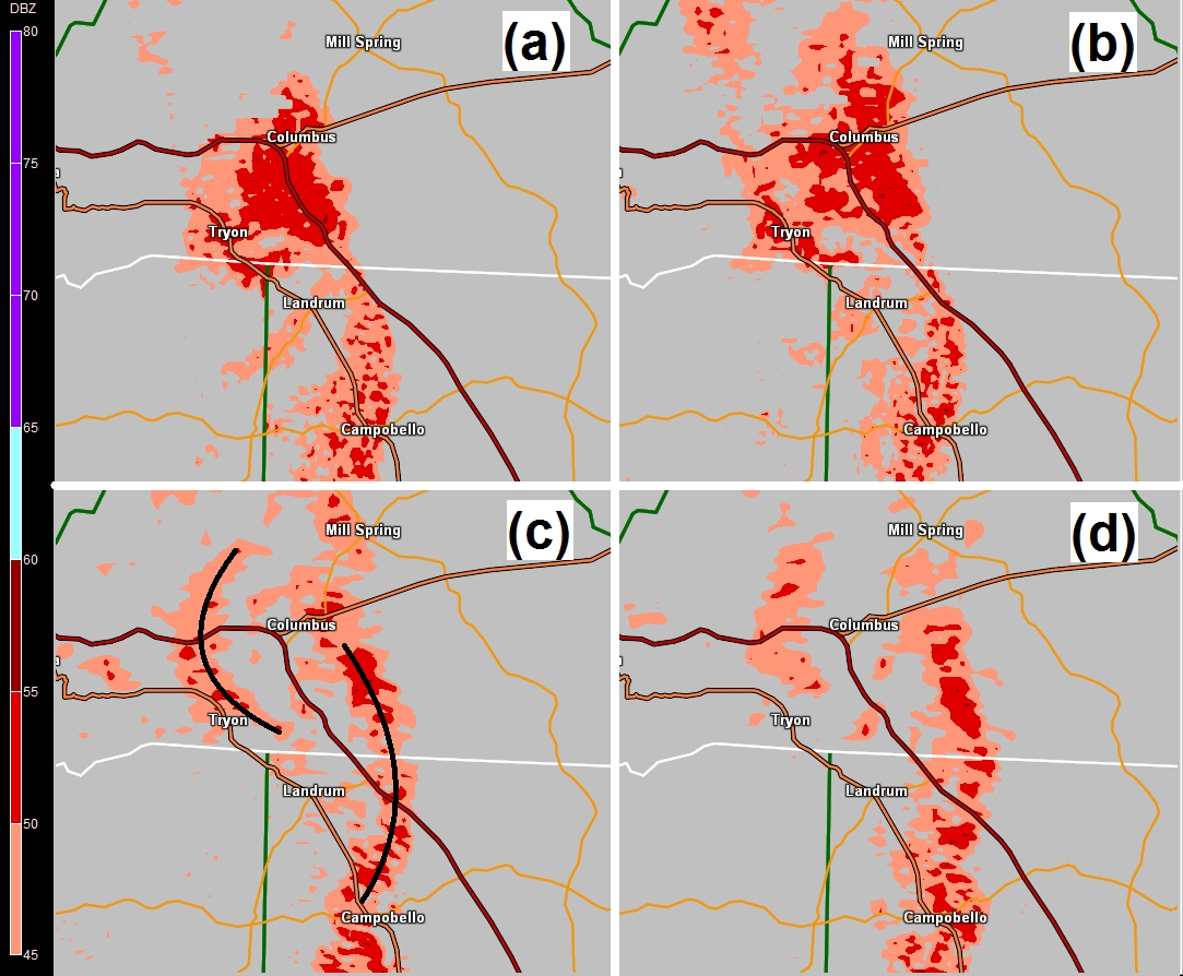
Fig. 33. As in Fig. 32, except with reflectivity less than 45 dBz filtered out and Broken-S signature delineated with black lines. Click to enlarge.

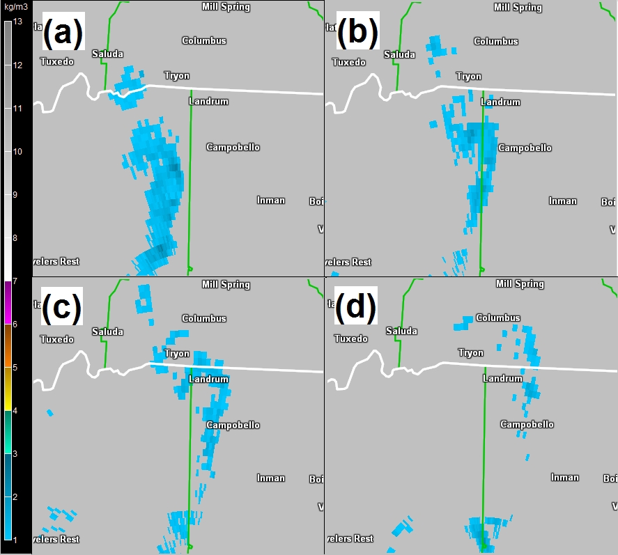
Fig. 34. VILD from KGSP at (a) 2354 UTC on 14 October 2015 and (b) 0005 UTC, (c) 0010 UTC, and (d) 0015 UTC on 15 October 2014. Click to enlarge.

A fully-formed "Broken-S" reflectivity signature was identified across northern Polk County, North Carolina, at 0028 UTC (Fig. 35). Isolating the higher reflectivity values highlighted the signature very well (Fig. 36). The fracture occurred roughly along the direction of the 0-3 km shear vector. While the reflectivity segment east of the fracture maintained a QLCS structure, the segment west of the fracture appeared as a discrete cell, although the reflectivity core was stretched along the direction of the mean cloud-bearing wind. This fairly classic evolution of HSLC convection was modeled by Weisman and Trapp (2003). They found that the reflectivity "fracture" began aloft in response to a downward-directed pressure gradient that developed above the mesovortex. In other words, the dynamics of this process were similar to that of splitting supercells. Weak tornadoes were common as the QLCS fractured. The reflectivity fracturing may be a visual clue that the mesovortex has reached a "tipping point" such that vorticity is strong enough to support tornadogenesis. Although the discrete cell was associated with cyclonic rotation, it was quite weak, as NROT peaked at 0.57 at 0.9 degrees (1.0 km AGL; Fig. 37).

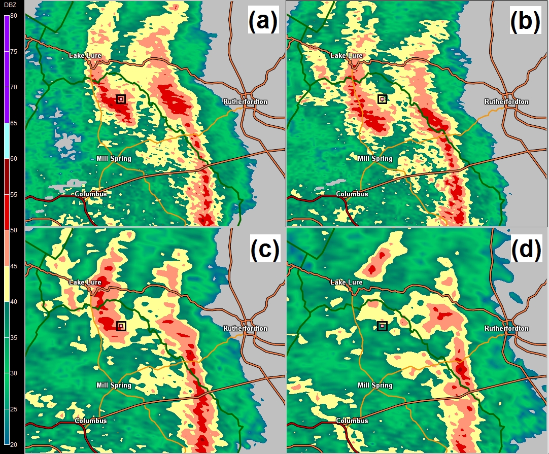
Fig. 35. KGSP base reflectivity at (a) 0.5 degrees at 0028 UTC, and (b) 0.9 degrees, (c) 1.8 degrees, and (d) 3.1 degrees at 0026 UTC on 15 October 2014. The pink square inside the black box indicates the location of the maximum NROT on the 0.5 degree scan. Click to enlarge.

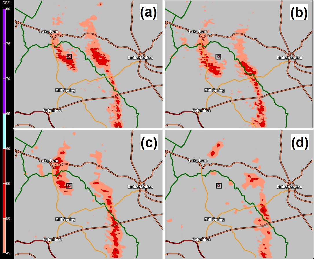
Fig. 36. As in Fig. 35, except with reflectivity less than 45 dBz filtered out. Click to enlarge.

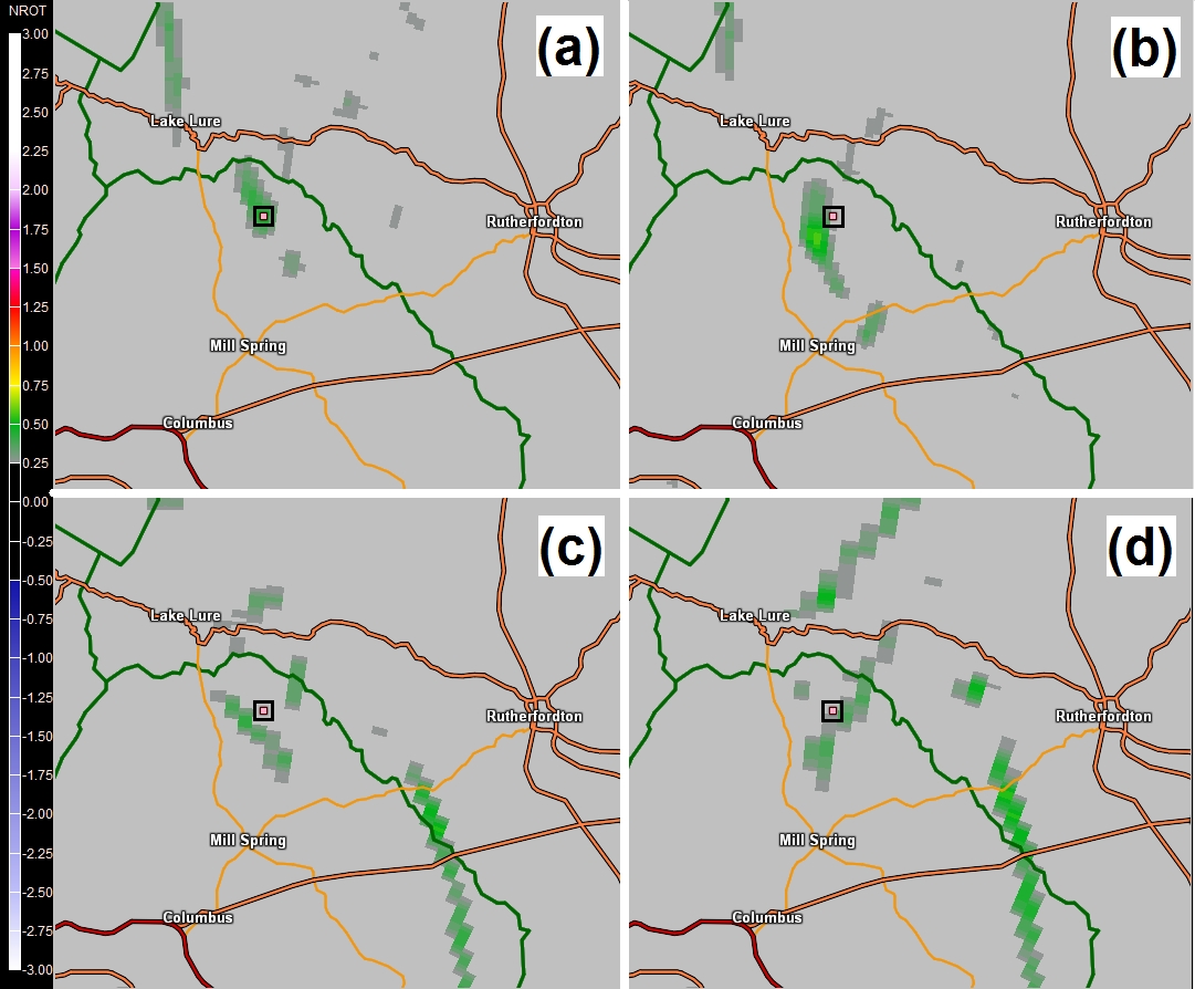
Fig. 37. As in Fig. 35, except for NROT. Click to enlarge.

c.  The Montford Cove Road (McDowell County) Tornado

The discrete cell remained steady-state as it moved across northwest Rutherford County, North Carolina, and exhibited persistent but weak rotation. The cell began to strengthen as it approached the McDowell County border, with 50 dBz echoes extending above 2.0 km ASL by 0042 UTC (Fig. 38). A concurrent increase in low level rotation (30% over the previous scan) was noted as well, as 0.5 degree NROT increased to 0.69 at 0045 UTC (Fig. 39) just a few minutes before another EF0 tornado developed over southern McDowell County. This was almost an hour after the Gowensville tornado. A similar behavior was noted in several CSTAR cases, has been documented in an HSLC study from the United Kingdom (Clark 2010), and has been observed with previous HSLC events in the GSP CWA, the most notable being the 15 November 2006 case. While past case studies of these events focused mainly on tornadoes that occurred near the time of the reflectivity fracture, additional, possibly more intense tornadoes have occurred with discrete cells that developed and persisted on the left (i.e., north or west) side of the reflectivity fracture. In similar cases, tornadogenesis has occurred 30 minutes or more after the Broken-S signature developed. Unfortunately, it has been unusual for these events to be accompanied by intense radar velocity signatures unless they were close to the radar.

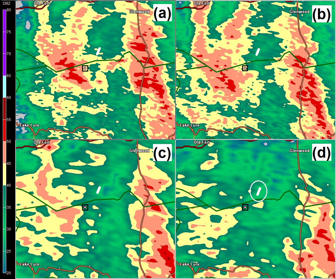
Fig. 38. KGSP base reflectivity on the (a) 0.5 degree scan at 0045 UTC, (b) 0.9 degree, (c) 1.8 degree, and (d) 3.1 degree scan at 0042 UTC on 15 October 2014. The green line is the boundary between Rutherford County (south) and McDowell County (north). The white line represents the track of the McDowell County tornado, circled in (d). The pink square inside the black box represents the location of the maximum NROT on the 0.5 degree scan. Click to enlarge.

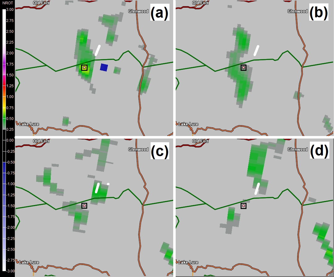
Fig. 39. As in Fig. 38, except for NROT. Click to enlarge.

It was notable that the McDowell County tornado occurred within a constricted region of a south-southwest to north-northeast oriented drainage (Cove Creek; Fig. 40). The elevation of the valley near the tornado location was around 335 m ASL (1100 ft), while the elevation of the surroundings hills on either side of the tornado track was around 610 m ASL (2000 ft; Fig. 41). Considering the orientation of the prevailing flow, low level winds may have accelerated through this channel, which would have enhanced storm relative helicity and inflow. This possibility was supported by output from the Wind Ninja program (Fig. 42). Given an input "ambient, flat surface" 10 m wind speed and direction, the program outputs high resolution, theoretical wind information, adjusting the surface wind based upon terrain. Potential terrain modification of the near-storm environmental flow has been noted in other tornado events across the foothills and valleys of the Southern Appalachians (e.g., Gaffin 2012; Schneider 2009; Gerapetritis 2000). It has also been a personal observation of the author that previously non-tornadic, steady-state storms within tornadic environments become more likely to produce tornadoes as they move from the Piedmont into the slightly more complex terrain of the foothills.

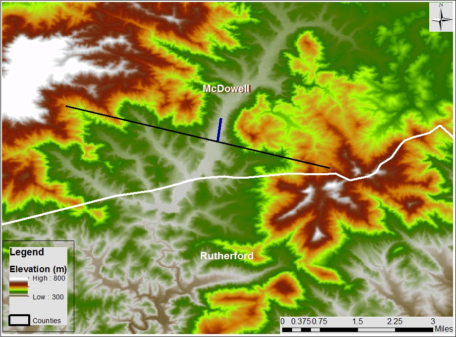
Fig. 40. Topographic map showing the track of the McDowell County tornado on 15 October 2014, shown as the thick blue line. The white line shows the boundary between McDowell County and Rutherford County. The thin black line shows the track of the terrain cross-section shown in Fig. 41. Click to enlarge.

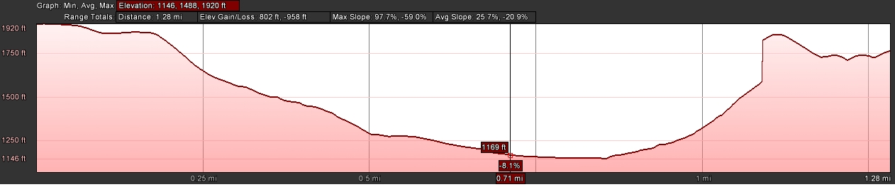
Fig. 41. Elevation cross section across the Cove Creek drainage and perpendicular to the path of the McDowell County tornado. The red arrow points to the position of the tornado track. The length of the cross section is about 2 km (1.3 miles). The lowest point in the drainage is about 349 m (1146 ft) MSL. The highest point on the surrounding ridges is 585 m (1920 ft) MSL. (Image from Google Earth). Click to enlarge.

Fig. 42. Same as in Fig. 40, except with an overlay of output from the Wind Ninja program. In this case, an ambient wind speed of 180 degrees at 19 kts was used as input. The image indicates the acceleration of flow that may have occurred through the Cove Creek drainage around 0000 UTC on 15 October 2014. Click to enlarge.

The environment became increasingly less favorable for additional severe weather to the north and east through the late evening hours. In fact, a report of wind damage near Marion, North Carolina, was the last occurrence of severe weather.

4. Discussion and Conclusions

Forecasters at WFO GSP correctly anticipated an increased threat of severe thunderstorms on 14 October 2014 through interpretation of numerical model guidance that depicted a favorable juxtaposition of a meridional jet streak, high-amplitude 500 hPa trough, sharp west-to-east moisture gradient, and strong meridional surface cold front. The outcome on 14 October was in contrast with three potential HSLC events during the previous three years (10 December 2012, 22 December 2013, and 14 April 2014) that did not meet expectations, in that little to no severe weather occurred across the GSP CWA. The environments on those days had weaker moisture gradients, southwest-to-northeast oriented surface cold fronts, and 500 hPa trough axes located along or west of the Mississippi River. This suggests the magnitude and orientation of synoptic scale forcing may play a role in discriminating between HSLC environments that produce severe weather and environments that do not.

The Western Carolina tornadoes of 14 October 2014 further illustrate the need to carefully analyze radar and environmental data during HSLC convective events. The NROT product in GR2Analyst is an effective way of evaluating trends in storm-scale shear and rotation, especially in rapidly changing situations such as HSLC events. Gust front boundaries oriented parallel to a radar beam will be revealed as elongated axes of cyclonic vertical vorticity. Any areas of rotation (i.e., a local inbound/outbound velocity couplet) that develop along this axis should arouse suspicion, especially if there is corroborating reflectivity clues, such as a forward flank notch and/or line echo wave pattern.  Significant increases in radar-indicated rotation were noted at 0.5 degrees in both events about five minutes prior to tornadogenesis (Fig. 43). 

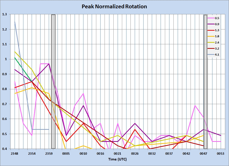
Fig. 43. Time series plot of NROT associated with tornadic cell at the indicated radar elevation angles between 2348 UTC on 14 October 2014 and 0053 UTC on 15 October 2014. Gray boxes delineate tornado times. Click to enlarge.

In the Gowensville Tornado case, the NROT product was the first radar product to clearly indicate that the QLCS, more specifically the gust front, was fracturing into two segments.  This was observed more than five minutes before the Gowensville tornado, and approximately 15 minutes before the Broken-S reflectivity signature was revealed at higher elevation scans.  The fracturing of the QLCS in the base reflectivity imagery will typically first be observed near the top of the high reflectivity core, and sometimes begins as a bulb of high reflectivity, with perhaps a relative reflectivity minimum in the middle of the bulb.  This is often the first clue that the core is beginning to separate into two segments.  Although the fracturing progressively works its way toward the surface, it may not be seen near the level of the cloud base until well after a tornado has occurred.  Therefore, the Broken-S signature, somewhat paradoxically, is more likely to be identified and provide some amount of tornadogenesis lead time when it is observed at medium-to-long range from the radar.  Closer to the radar, more data (i.e., more than the lowest four elevation slices) must be analyzed to identify developing Broken-S signatures. The digital VIL product, used in conjunction with base data, can also be helpful in analyzing weakening of radar echoes in the vicinity of mesovortices.

Acknowledgments

Upper air analyses, thermodynamic diagrams, and mesoanalyses were obtained from the NOAA/NWS Storm Prediction Center. Surface analyses were obtained from the NOAA/NWS Weather Prediction Center. The radar mosaic and satellite imagery were obtained from the University Corporation for Atmospheric Research\NCAR Real-Time Weather Data web page.  The RAP model forecast sounding plot was created using the RAwinsonde OBservation (RAOB) Program for Windows.  Local radar graphics were created using GR2Analyst version 2.22 for Windows.

References

Clark, M. R., 2009:  The southern England tornadoes of 30 December 2006: Case study of a tornadic storm in a low CAPE, high shear environment.  Atmos. Res., 93, 50–65,

Clark, M. R., 2011:  Doppler radar observations of mesovortices within a cool-season tornadic squall line over the UK.  Atmos. Res., 100, 749-764.

Davis, J. M., and M. D. Parker, 2014:  Radar climatology of tornadic and non-tornadic vortices in high shear, low CAPE environments in the mid-Atlantic and southeastern U.S. Wea. Forecasting, 29, 828-853.

Evans, M., 2010:  An examination of low CAPE/high shear severe convective events in the Binghamton, New York, county warning area.  Natl. Wea. Dig., 34, 129–144.

Gaffin, D. M., 2012:  The influence of terrain during the 27 April 2011 Super Tornado Outbreak and 5 July 2012 derecho around the Great Smoky Mountains National Park.  Preprints, 26th Conf. on Severe Local Storms, Nashville, TN, Amer. Meteor. Soc.

Gerapetritis, H., 2000:  Short-term forecasting of tornadic environments in the complex terrain of western North Carolina.  Preprints, 20th Conf. Severe Local Storms, Orlando, FL, Amer. Meteor. Soc., 567-570.

King, J. R., and M. D. Parker, 2014:  Synoptic influence on High Shear, Low CAPE convective events.  Preprints, 27th AMS Conf. on Severe Local Storms, Madison, WI, Amer. Meteor. Soc.

Lane, J. D., and P. D. Moore, 2006:  Observations of a non-supercell tornadic thunderstorm from terminal Doppler weather radar.  Preprints, 23rd Conf. on Severe Local Storms, St.Louis, MO, Amer. Meteor. Soc., P4.5.

Schneider, D. G., 2009:  The impact of terrain on three cases of tornadogenesis in the Great Tennessee Valley.  J. Operational Meteor., 10 (11), 1–33.

Sherburn, K. D., and M. D. Parker, 2014:  Climatology and ingredients of significant severe convection in high shear, low CAPE environments.  Wea. Forecasting, 29, 854-877.

Trapp, R. J., and M. L. Weisman, 2003:  Low-level mesovortices within squall lines and bow echoes: Part II. Their genesis and implications.  Mon. Wea. Rev., 131, 2804-2823.